In this last blog post in our series we explore in detail the characteristics of various high quality re-rankers including our own Elastic Rerank model. In particular, we focus on qualitative and quantitative evaluation of retrieval quality as a function of reranking depth. We provide some high-level guidelines for how to select reranking depth and recommend reasonable defaults for the different models we tested. We employ a "retrieve-and-rerank" pipeline using BM25 as our first stage retriever. We focus on English language text search and use BEIR to benchmark our end-to-end accuracy.
Summary
Below we show that end-to-end relevance follows three broad patterns as a function of re-ranking depth:
- Fast increase followed by saturation
- Fast increase to a maximum then decay
- Steady decay with any amount of re-ranking
For the re-rankers and datasets tested pattern 1 accounted for around 72.6% of all results, followed by pattern 2 (20.2%) and then pattern 3 (7.1%). Unsurprisingly the overall strongest re-rankers, such as Elastic Rerank, display the most consistent improvements with re-ranking depth.
We propose a simple model which explains the curves we observe and show it provides a surprisingly good fit across all datasets and re-rankers we tested. This suggests that the probability of finding a positive document at a given depth in the retrieval results follows a Pareto distribution. Furthermore, we can think of the different patterns being driven by the fraction of relevant (or positive) documents the re-ranker can detect and the fraction of irrelevant (or negative) documents it mistakenly identifies as relevant.
We also study effectiveness versus efficiency as a mechanism to choose the re-ranking depth and to perform model selection. In the case there is no hard efficiency constraint, as a rule-of-thumb we pick the depth that attains 90% of the maximum effectiveness. This yields a 3× improvement in compute cost compared to maximizing effectiveness, so we feel it represents a good efficiency tradeoff. For our benchmark, the 90% rule suggests one should re-rank around 100 pairs from BM25 on average, although stronger models give more benefit from deeper re-ranking. We also observe an important first stage retrieval effect. For some data sets we study the retriever recall saturates at a relatively low depth. In those scenarios we see significantly shallower maximum and 90% effectiveness depths.
In the realistic scenarios there are efficiency constraints, such as the maximum permitted query latency or compute cost. We propose a scheme to simultaneously select the model and re-ranking depth subject to an efficiency constraint. We find that when efficiency is at a premium, deep re-ranking with small models tends to out perform shallow re-ranking with larger higher quality models. This pattern reverses as we relax the efficiency constraint. We also find that Elastic Rerank provides state-of-the-art effectiveness versus efficiency, being optimal for nearly all constraints we test. For our benchmark we found re-ranking around the top 30 results from BM25 represented a good choice when compute cost is important.
The re-rankers
For this investigation we evaluate a collection of re-rankers of different sizes and capabilities. More specifically:
- Elastic Rerank: This was trained from a DeBERTa V3 base model checkpoint. We discussed some aspects of its training in our last post. It has roughly 184M parameters (86M in the "backbone" + 98M in the input embedding layer). The large embedding parameter count is because the vocabulary is roughly 4× the size of BERT.
- bge-reranker-v2-gemma: This is an LLM based re-ranker trained on one of the Google Gemma series of models. It’s one of the strongest re-ranking models available and has around 2B parameters.
- monot5-large: This is a model trained on the MS MARCO passage dataset using T5-large as backbone. At the time of release it demonstrated state-of-the-art zero shot performance and it’s still one of the strongest baselines. It has around 770M parameters.
- mxbai-rerank-base-v1: This model is provided by Mixedbread AI and according to the company’s release post it was trained by a) first collecting the top-10 results from search engines for a large number of queries, b) asking a LLM to judge the results for their relevance to the query and finally c) using these examples for training. The model uses the same DeBERTa architecture as the Elastic Reranker.
- MiniLM-L12-v2: This is a cross-encoder model trained on the MS MARCO passage ranking task. It follows the BERT architecture with around 33M parameters.
- Cohere-v3: This is an efficient and high quality commercial re-ranker provided by Cohere. No further information is available regarding the parameter count for this model.
Oracle
In the graphs below we include the performance of an "oracle" that has access to the relevance judgments (qrels) per dataset and thus can sort the documents by their relevance score descending. This puts any relevant document before any irrelevant document and higher relevance documents higher than lower relevance ones. These data points represent the performance of the ideal re-ranker (assuming perfect markup) and quantify the available space of improvement for the re-ranking models. It also captures the dependence of the end-to-end accuracy on the first stage retriever as the re-ranker only has visibility over the items that the retriever returns.
Main patterns
We use nDCG@10 as our evaluation metric, which is the standard in the BEIR benchmark, and we plot these scores as a function of the re-ranking depth. Re-ranking depth is the number of candidate documents retrieved by BM25 and subsequently sent to the re-ranker. Since we are using nDCG@10 the score is affected only when a document that is found lower in the retrieved list is placed in the top-10 list by the re-ranker. In this context, it can either increase nDCG@10 if it is relevant or it can evict a relevant document and decrease nDCG@10.
In the following we describe the main patterns that we identified in these graphs across the different combinations of datasets and models we tested. We present them in decreasing order of frequency and provide some possible explanations of the observed behavior.
"Pareto" curve
This accounts for most of the cases that we see. It can be divided into three phases as follows:
- Phase A: A rapid increase which takes place mostly at smaller depths (< 100)
- Phase B: Further improvements at a smaller rate
- Phase C: A "plateau" in performance
Below you can see runs from DBpedia and HotpotQA, where the black dashed horizontal line depicts the nDCG@10 score of BM25
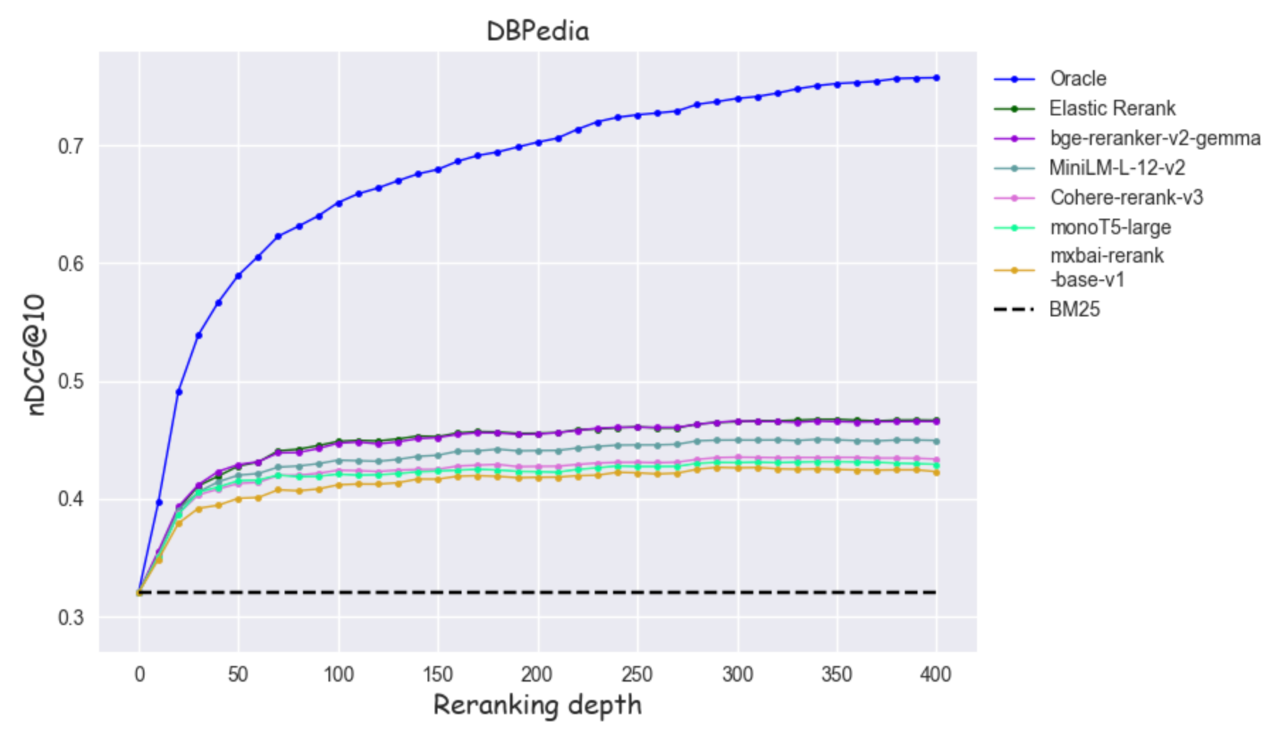
Figure 1: nDCG@10 as a function of reranking depth on DBpedia
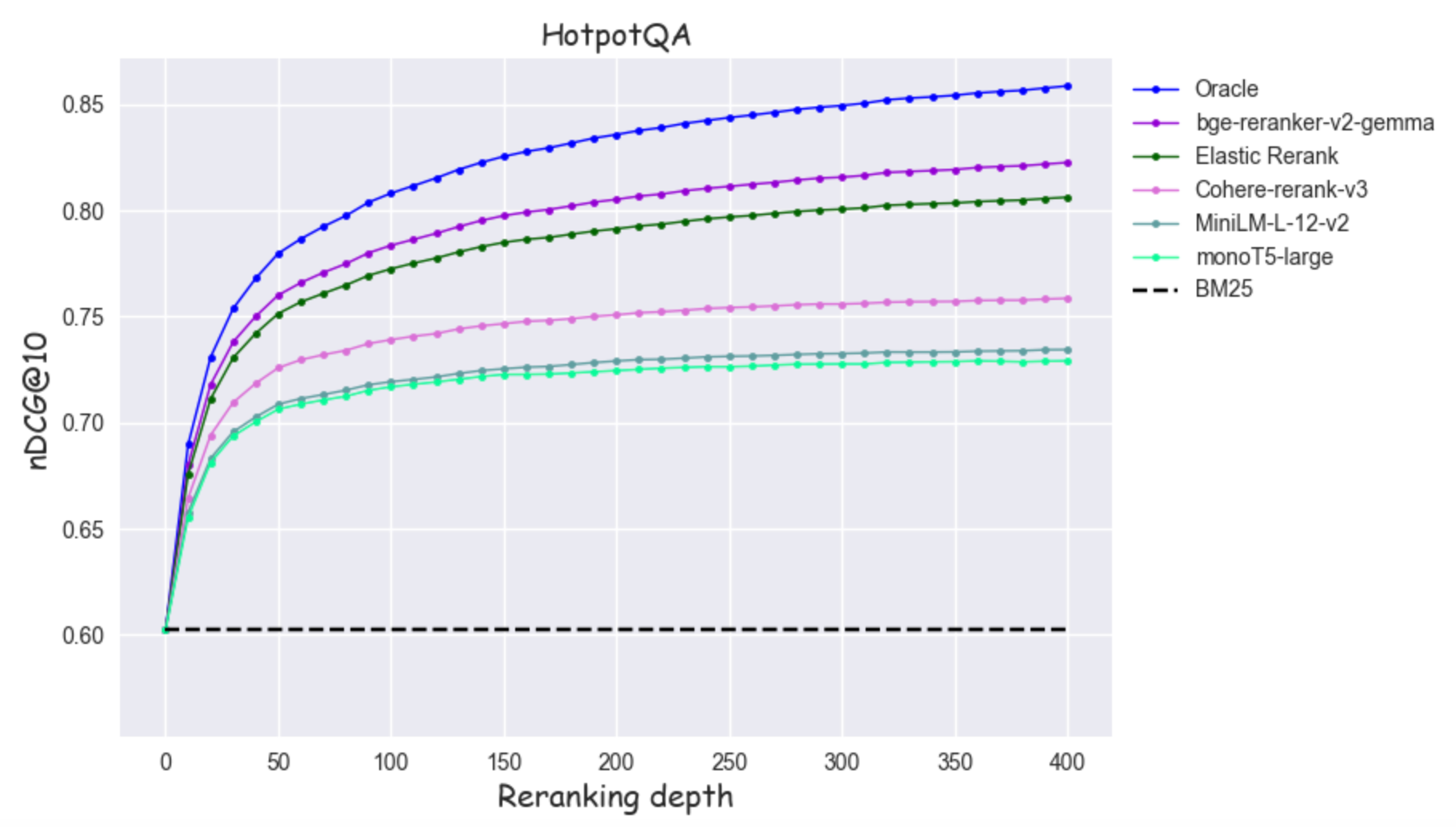
Figure 2: nDCG@10 as a function of reranking depth on HotpotQA
Discussion
A monotonically increasing curve has a simple explanation: as we increase the re-ranking depth, the first-stage retriever provides a larger pool of candidates to the next stage so that the re-ranker models can identify additional relevant documents and place them high in the result list.
Based on the shape of these curves, we hypothesize that the rate at which we discover positives as a function of depth follows a power law. In particular, if we assume that the re-ranker moves each positive into the top-10 list, nDCG@10 will be related to the count of positives the retriever returns in total for a given depth. Therefore, if our hypothesis is correct its functional form would be related to the cumulative density function (CDF) of a power law. In the following, we fit a scaled version of a generalized Pareto CDF to the nDCG@10 curves to test this hypothesis.
Below you can see some examples of fitted curves applied to a selection of datasets (FiQA, Natural Questions, DBpedia and HotpotQA) using different re-rankers.
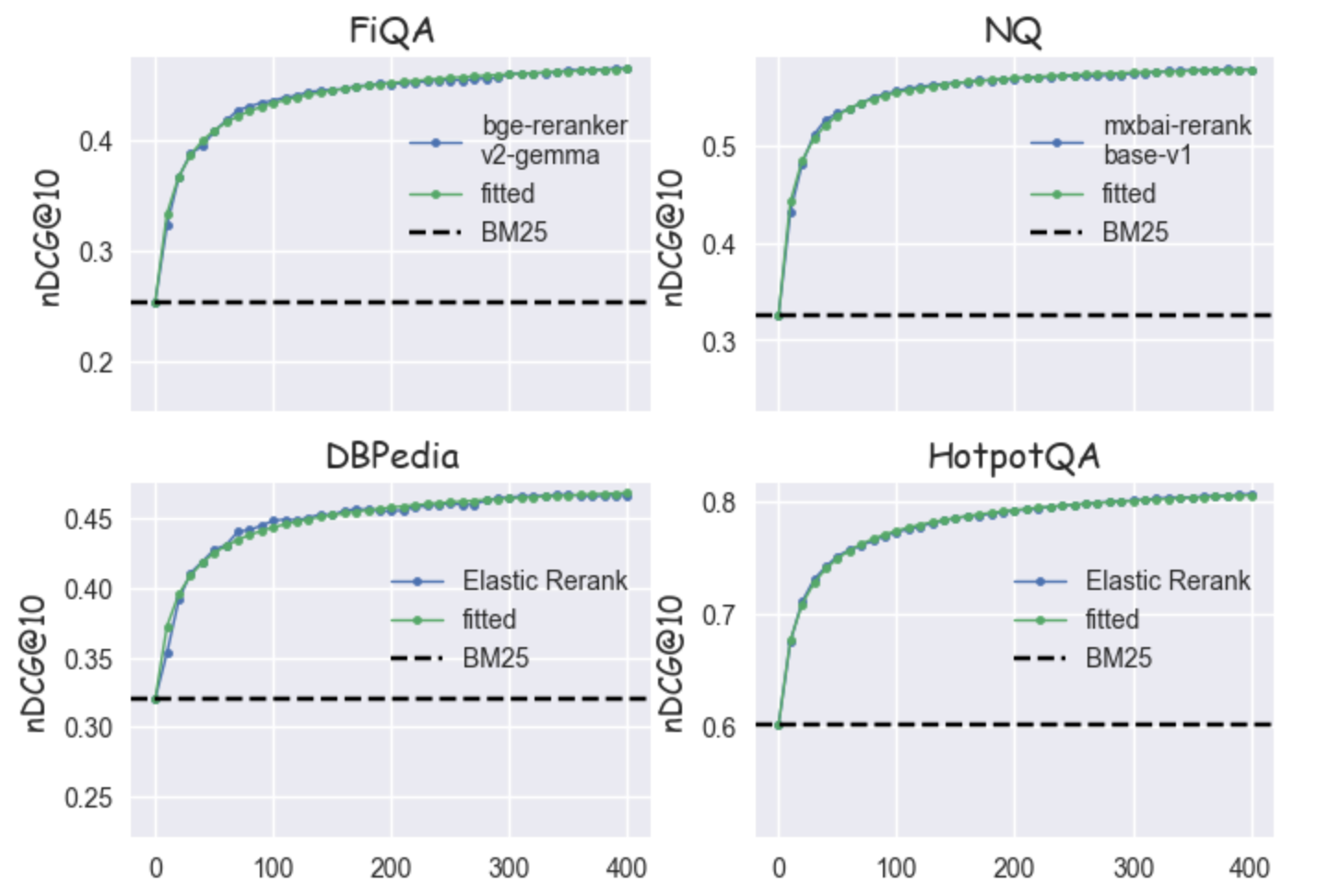
Figure 3: Curve fitting of the nDCG graph using a generalized Pareto CDF
Visually it is clear that the generalized Pareto CDF is able to fit the observed curves well, which supports our hypothesis.
Since we don’t match the performance of the oracle the overall behavior is consistent with the model having some false negative (FN) fraction, but a very low false positive (FP) fraction: adding more examples will occasionally shuffle an extra positive to the top, but won’t rank a negative above the positives found so far.
"Unimodal" curve
This family of graphs is characterized by the following phases:
- Phase A: Rapid increase until the peak
- Phase B: Performance decrease at a smaller rate
Below you can see two examples of this pattern: one when the MiniLM-L12-v2 model is applied on to the TREC-COVID dataset and a second when the mxbai-rerank-base-v1 model is applied to the FEVER dataset. In both cases, the black dashed line represents the performance of the BM25 baseline
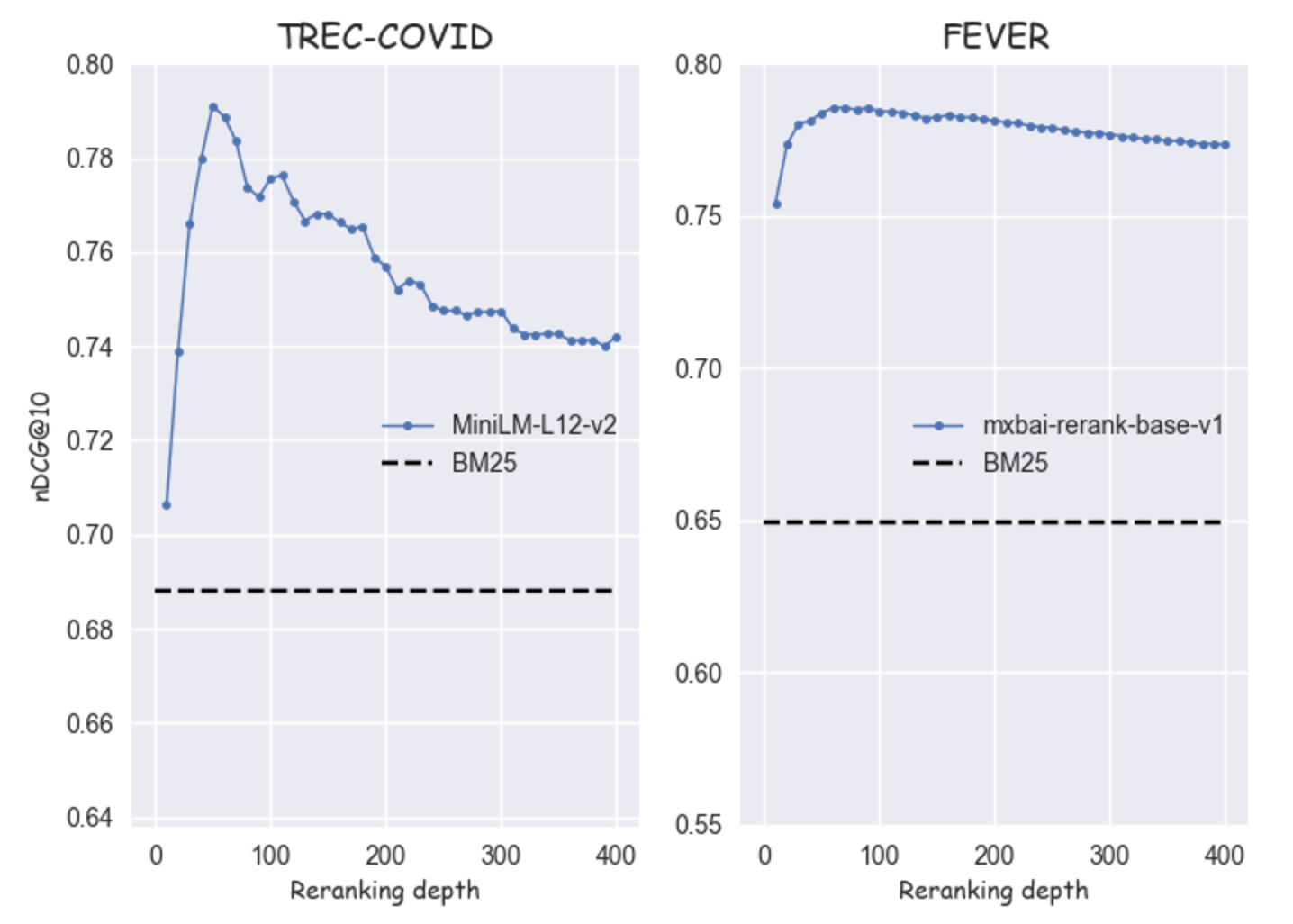
Figure 4: Two cases of the "unimodal" pattern
Discussion
This sort of curve would be explained by exactly the same Pareto rate of discovery of extra relevant documents. However, it also appears there is some small non-zero FP fraction. Since the rate of discovery of additional relevant documents decreases monotonically, at a certain depth the rate of discovery of relevant documents multiplied by the true positive (TP) fraction will equal the rate of discovery of irrelevant documents multiplied by the FP fraction and the nDCG@10 will have a unique maximum. Thereafter, it will decrease because in aggregate re-ranking will push relevant documents out of the top-10 set.
There are some likely causes for the presence of a non-zero FP rate:
- Incomplete markup: In other words the model surfaces items which are actually relevant, but not marked as such which penalizes the overall performance. This is something we have investigated in a previous blog.
- Re-ranker training: Here, we broadly refer to issues that have to do with the training of the re-ranker. One possible explanation is provided in this paper by Gao et al. where the authors emphasize the importance of tailoring a re-ranker to the retriever because there might be cases where false positives at lower positions share confounding characteristics with the true positives which ultimately "confuses" the re-ranker.
However, we note that this pattern is more common for overall weaker re-ranking models.
As we discussed in our previous blog, a potential mitigation for training issues in a zero-shot setting is to ensure that we present sufficiently diverse negatives to cover a broad set of possible confounding features. In other words, it could be the case that models which exhibit these problems haven’t mined enough deep negatives for training and thus deeper retrieval results are effectively "out-of-domain".
Note that there are some edge cases where it’s hard to distinguish between the "Pareto" and "Unimodal" patterns. This happens when the peak in performance is achieved earlier than the maximum depth but the performance decrease is marginal. Based on the terminology used so far this would qualify as a "Unimodal" case. To address this, we introduce this extra rule: we label curves as "Pareto" if their nDCG gain at maximum depth is ≥ 95% of the maximum nDCG gain and "Unimodal" otherwise.
Bad fit
This category comprises all cases where the application of a re-ranker does not bring a performance benefit at any depth compared to BM25. On the contrary, we observe a continuous degradation as we re-rank more documents.
As an example we can take ArguAna, which is a particularly challenging task in BEIR as it involves the retrieval of the best counterargument to the input. This is not a typical IR scenario and some studies even consider reporting results without it. We experimented with different re-rankers (even with some that didn’t make it into the final list) and we observed that many of them (Cohere-v3, bge-reranker-v2-gemma and Elastic Rerank being the only exceptions) exhibited the same pattern. Below we show the results for monot5-large.
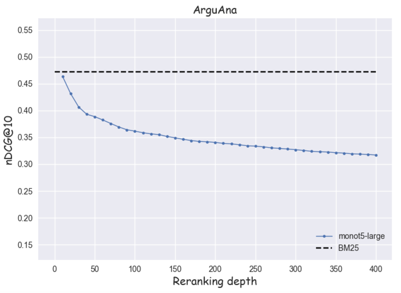
Figure 5: A "bad-fit" example
Discussion
We propose two possible explanations:
- The re-ranker could be a bad fit for the task at hand, which is sufficiently out of the training domain that its scoring is often incorrect,
- The re-ranker could just be worse than BM25 for the particular task. BM25 is a strong zero-shot baseline, particularly for certain query types such as keyword searches, because it relies on lexical matching with scoring tailored to the whole corpus.
Overview of patterns
Overall, the distribution of the patterns (P → "Pareto" curve, U → "Unimodal" curve, B → "Bad fit") across all scenarios is as follows:
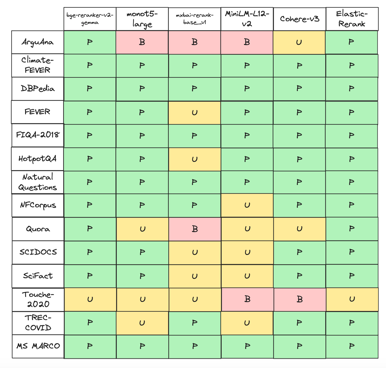
Figure 6: Distribution of patterns across all scenarios
Regarding the "Pareto" pattern which is by far the most common, we note some observations from relevant works. First, this paper from Naver Labs presents results which are in line with our findings. There, the authors experiment with 3 different (SPLADE) retrievers and two different cross-encoders and test the pipeline on TREC-DL 19, 20 and BEIR. They try three different values for the re-ranking depth (50, 100 and 200) and the results show that in the majority of the cases the performance increases at a rapid pace at smaller depths (i.e. 50) and then almost saturates. A relevant result is also presented in this blog post from Vespa where the author employs a "retrieve-and-rerank" pipeline using BM25 and ColBERT on the MLDR dataset and finds that the nDCG metric can be improved significantly by re-ordering just the top ten documents. Finally, in this paper from Meng et al. we observe similar results when two retrieval systems (BM25 and RepLLaMA) are followed by a RankLLaMA re-ranker. The authors perform experiments on the TREC DL19 and 20 datasets investigating 8 Ranked List Truncation (RLT) methods, one of which is "Fixed-k" that aligns with our setup. In none of these works do the authors identify an explicit underlying process that could explain the observed nDCG curve. Since we found the behavior was consistent with our simple model across different datasets and re-rankers this feels like it warrants further investigation.
Some characteristics of the other retrieval tasks that could also explain some of these results:
ArguAnaandTouche-2020, both argument retrieval datasets, present the most challenging tasks for the models we consider here. An interesting related analysis can be found in this paper by Thakur et al. where the authors discuss the reduced effectiveness of neural retrieval models inTouche-2020especially when compared to BM25. Even though the paper considers a single retrieval step we think that some of the conclusions might also apply to the "retrieve-and-rerank" pipeline. More concretely, the authors reveal an inherent bias of neural models towards preferring shorter passages (< 350 words) in contrast to BM25 which retrieves longer documents (>600 words) mimicking the oracle distribution better. In their study, even after "denoising" the dataset by removing short docs (less than 20 words) and adding post-hoc relevance judgments to tackle the small labeling rate BM25 continues to outperform all the retrieval models they tested.ScifactandFEVERare two datasets where two of the "smaller" models follow "unimodal" patterns. Both are fact verification tasks which require knowledge about the claim and reasoning over multiple documents. On Scifact it is quite important for the retriever to be able to access scientific background knowledge and make sense of specialized statistical language in order to support or refute a claim. From that perspective smaller models with less internal "world" knowledge might be at disadvantage.- According to our previous study
TREC-COVIDhas a large labeling rate i.e. for >90% of the retrieved documents there is a relevance judgment (either positive or negative). So, it’s the only dataset where incomplete markup is not likely a problem. - BM25 provides very good ranking for
Quora, which is a "duplicate questions" identification task. In this particular dataset, queries and documents are very short - 90% of the documents (queries) are less than 19 (14) words - and the Jaccard similarity across queries and their relevant counterparts is quite high, a bit over 43%. This could explain why certain purely semantic re-rankers can fail to add value.
Understanding scores as a function of depth
So far we treated a re-ranker model as though it were a classifier and discussed its performance in terms of its FN and FP rates. Clearly, this is a simplification since it outputs a score which captures some estimate of the relevance of each document to the query. We return to the process of creating interpretable scores for a model, which is called calibration, in a separate upcoming blog post. However, for our purposes here we would like to understand the general trends in the score as a function of depth because it provides further insight into how the nDCG@10 evolves.
In the following figures we split documents by their judgment label and plot the average positive and negative document scores as a function of depth for examples from the three different patterns we identified. We also show one standard deviation confidence intervals to give some sense of the overlap of score distributions.
For the Pareto pattern we see positive and negative scores follow a very similar curve as depth increases. (The negative curve is much smoother because there are many more negatives at any given depth.) They start higher, a regime which corresponds to excellent matches and very hard negatives, then largely plateau. Throughout the score distributions remain well separated, which is consistent with a FP fraction which is essentially zero. For the unimodal pattern there is a similar decay of scores with depth, but we also see noticeably more overlap in the score distributions. This would be consistent with a small but non-zero FP fraction. Finally, for the bad fit pattern we see that scores are not separated. Also there is no significant decrease in both the positive and negative scores with depth. This is consistent with the re-ranker being a bad fit for that particular retrieval task since it appears to be unable to reliably differentiate positives and negatives sampled from any depth.
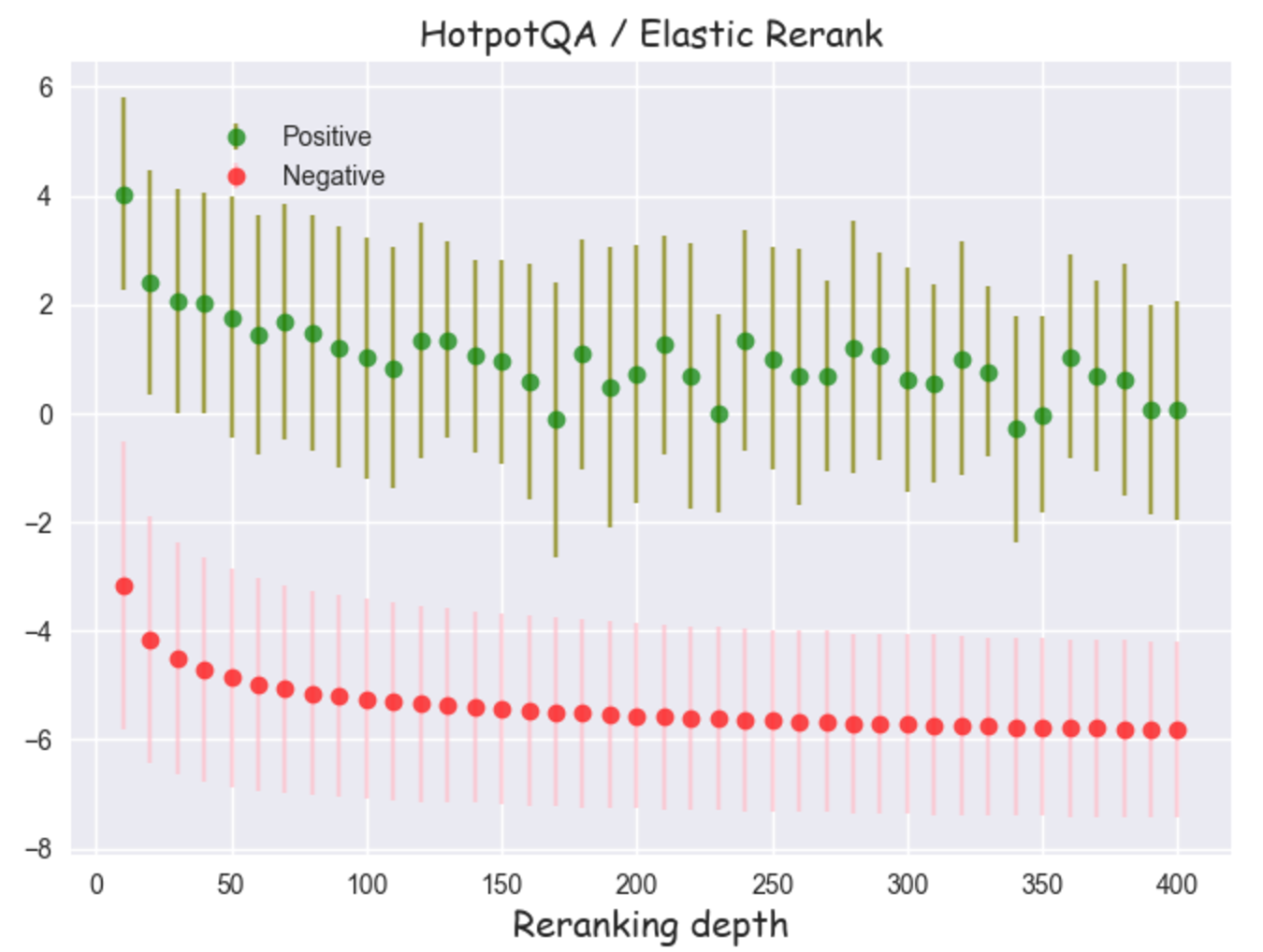
Figure 7: Positive and negative scores as a function of re-ranking depth for Elastic Rerank on HotpotQA. The bars correspond to ± 1 standard deviation intervals
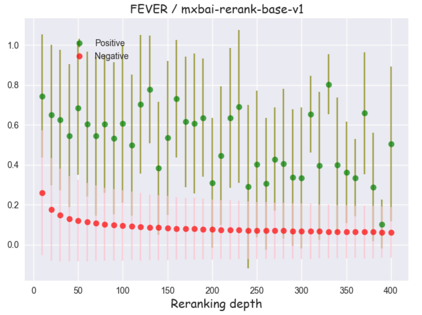
Figure 8: Positive and negative scores as a function of re-ranking depth for mxbai-rerank-base-v1 on FEVER. The bars correspond to ± 1 standard deviation intervals
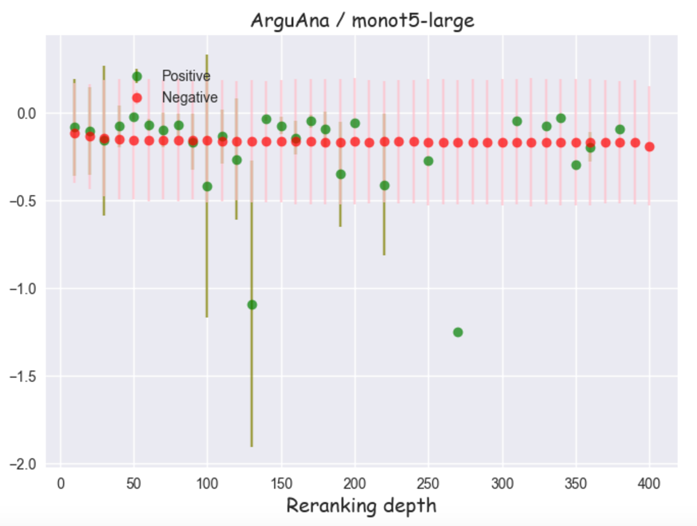
Figure 9: Positive and negative scores as a function of re-ranking depth for monot5-large on ArguAna. The bars correspond to ± 1 standard deviation intervals
Finally, note that the score curves for the unimodal pattern hints that one may be able to find a cut off score which results in a higher FN fraction but essentially zero FP fraction. If such a threshold can be found it would allow us to avoid the relevance degrading with re-ranking depth while still being able to retain a portion of the extra relevant documents the retriever surfaces. We will return to this observation in an upcoming blog post when we explore model calibration.
Efficiency vs effectiveness
In this section we focus on the trade-off between efficiency and effectiveness and provide some guidance on picking optimal re-ranking depths. At a high level, effectiveness refers to the overall gain in relevance we attain as we retrieve and re-rank more candidates, while efficiency focuses on minimizing the associated cost.
Efficiency can be expressed in terms of different dimensions with some common choices being:
- Latency, which is usually tied to an SLA on the query duration. In other words, we may only be allowed a fixed upper wall time for re-scoring (query, document) pairs, and
- Infrastructure cost, which refers to the number of CPUs/GPUs needed to keep up with the query rate or the total compute time required to run all queries in a pay-as-you-go setting.
We note that efficiency is also wrapped up with other considerations such as the ability to run the model at lower precision, the ability to use more efficient kernels and so on, which we do not study further.
Here, we adopt a simplified setup where we focus solely on the latency dimension. Obviously, in a real-world scenario one could easily trade cost (i.e. by increasing the number of CPUs/GPUs and parallelising inference) to achieve lower latency, but for the rest of the analysis we assume fixed infrastructure.
Cohere v3 is excluded from this experimentation as it is an API-based service
"Latency-free" analysis
We start our analysis by considering each (model, dataset) pair in isolation ignoring the latency dimension. We are interested in the evolution of the nDCG gain (nDCG score at depth k minus the nDCG score of BM25) and we pick two data points for further analysis:
- The maximum gain depth, which is the re-ranking depth where the nDCG gain is maximized, and
- The 90%-depth, which corresponds to the depth where we first attain 90% of the maximum gain. This can be seen as a trade-off between efficiency and effectiveness as we get most of the latter at a smaller depth.
We calculate these two quantities across a selection of datasets.
| Dataset | DBPedia | HotpotQA | FiQA | Quora | TREC-COVID | Climate-FEVER | ||||||
|---|---|---|---|---|---|---|---|---|---|---|---|---|
| Model | max | 90% | max | 90% | max | 90% | max | 90% | max | 90% | max | 90% |
| bge-reranker-v2-gemma | 300 | 150 | 400 | 180 | 390 | 140 | 350 | 40 | 110 | 50 | 290 | 130 |
| monot5-large | 350 | 100 | 400 | 100 | 400 | 130 | 80 | 20 | 110 | 60 | 280 | 60 |
| MiniLM-L12-v2 | 340 | 160 | 400 | 120 | 400 | 80 | 20 | 20 | 50 | 50 | 280 | 50 |
| mxbai-rerank-base-v1 | 290 | 140 | 90 | 30 | 400 | 70 | 0* | 0* | 110 | 50 | 290 | 120 |
| Elastic Rerank | 350 | 140 | 400 | 160 | 400 | 130 | 180 | 30 | 220 | 50 | 400 | 170 |
| Cohere v3 | 300 | 100 | 400 | 130 | 400 | 130 | 30 | 20 | 270 | 50 | 290 | 70 |
Table 1: Max-gain and 90%-gain depths for different models and datasets. The "0* - 0*" entry for `mxbai-rerank-base-v1` on `Quora` indicates that the model does not provide any gain over BM25.
If we group by the re-ranker model type and average, it gives us Table 2. We have omitted the (Quora, mxbai-rerank-base-v1) pair as it corresponds to a bad-fit case.
| Model | Average of maximum gain depth | Average of 90%-to-max gain depth |
|---|---|---|
| bge-reranker-v2-gemma | 306.7 | 115 |
| monot5-large | 270 | 78.3 |
| MiniLM-L12-v2 | 248.3 | 80 |
| mxbai-rerank-base-v1 | 236 | 82 |
| Elastic Rerank | 325 | 113.3 |
| Cohere v3 | 281.7 | 83.3 |
Table 2: Average values for the depth of maximum gain and depth for 90% of maximum gain per model.
We observe that:
- More effective models such as
Elastic Rerankandbge-reranker-v2-gemmareach a peak performance at larger depths, taking advantage of more of the available positives, while less effective models "saturate" faster. - Obtaining 90% of the maximum gain is feasible at a much smaller depth in all scenarios: on average we have to re-rank 3× fewer pairs. A re-ranking depth of around 100 would be a reasonable choice for all the scenarios considered.
Alternatively, if we group by dataset and average we get Table 3.
| Model | Average of maximum gain depth | Average of 90%-to-max gain depth |
|---|---|---|
| DBPedia | 321.7 | 131.7 |
| HotpotQA | 348.3 | 120 |
| FiQA | 398.3 | 113.3 |
| Quora | 132 | 26 |
| TREC-COVID | 145 | 51.7 |
| Climate-FEVER | 305 | 100 |
Table 3: Average values per dataset.
There are two main groups:
- One group where the maximum gain depth is on average larger than 300. In this category belong
DBpedia,HotpotQA,FiQAandClimate-FEVER. - Another group where the maximum gain depth is significantly smaller - between 100 and 150 - containing
QuoraandTREC-COVID.
We suggest that this behavior can be attributed to the performance of the first stage retrieval, in this case BM25. To support this claim, we plot the nDCG graphs of the "oracle" below. As we know the nDCG metric is affected by a) the recall of relevant documents and b) their position in the result list. Since the "oracle" has perfect information regarding the relevance of the retrieved documents, its nDCG score can be viewed as a proxy for the recall of the first-stage retriever.
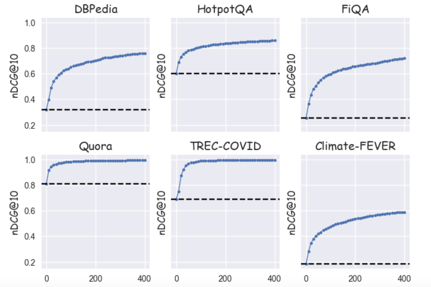
Figure 10: nDCG@10 curves for the "oracle" across different datasets
In this figure we see that for Quora and TREC-COVID the nDCG score rises quite fast to the maximum (i.e. 1.0) while in the rest of the datasets the convergence is much slower. In other words when the retriever does a good job surfacing all relevant items at shallower depths then there is no benefit in using a large re-ranking depth.
"Latency-aware" analysis
In this section we show how to perform simultaneous model and depth selection under latency constraints. To collect our statistics we use a VM with 2 NVIDIA T4 GPUs. For each dataset we measure the total re-ranking time and divide it by the number of queries in order to arrive into a single quantity that represents the time it takes to re-score 10 (query, document) pairs
We assume the cost is linearly proportional to depth, that is it takes s seconds to re-rank 10 documents, 2×s to re-rank 20 documents and so on.
The table below shows examples from HotpotQA and Climate-FEVER with each entry the number of seconds required to re-score 10 (query, document) pairs.
| Model | MiniLM-L12-v2 | mxbai-rerank-base-v1 | Elastic Rerank | monot5-large | bge-reranker-v2-gemma |
|---|---|---|---|---|---|
| HotpotQA | 0.02417 | 0.07949 | 0.0869 | 0.21315 | 0.25214 |
| Climate-FEVER | 0.06890 | 0.23571 | 0.23307 | 0.63652 | 0.42287 |
Table 4: Average time to re-score 10 (query, doc) pairs on HotpotQA & Climate-FEVER
Some notes:
mxbai-rerank-base-v1andElastic Rerankhave very similar running times because they use the same "backbone" model, DeBERTa- In most datasets
monot5-largeandbge-reranker-v2-gemmahave similar run times even thoughmonot5-largeonly has 1 / 3 the parameter count. There are two possible contributing factors:- For
bge-reranker-v2-gemmawe used bfloat16 while we kept float precision formonot5-large, and - The Gemma architecture is able to better utilize the GPUs.
- For
T-shirt sizing
The run times for different datasets can vary a lot due to the fact that queries and documents follow different length distributions. In order to establish a common framework we use a "t-shirt" approach as follows:
- We define the "Small" size as the time it takes the most efficient model (here
MiniLM-L-12-v2) to reach 90% of its maximal gain, similar to our proposal in the previous section, - We set other sizes in a relative manner, e.g. "Medium" and "Large" being 3x and 6x times the "Small" latency, respectively.
The model and depth selection procedure is best understood graphically. We create graphs as follows:
- On the X-axis we plot the latency and on the Y-axis nDCG@10
- The data points correspond to increments of 10 in the re-ranking depth, so more efficient models have a higher density of points in latency
- The vertical lines show the latency thresholds associated with the different "t-shirt" sizes
- For each model we print the maximum "permitted" re-ranking depth. This is the largest depth whose latency is smaller than the threshold
For each "t-shirt size" we simply pick the model and depth which maximizes the nDCG@10. This is the model whose graph has the highest intercept with the corresponding threshold line. The optimal depth can be determined by interpolation.
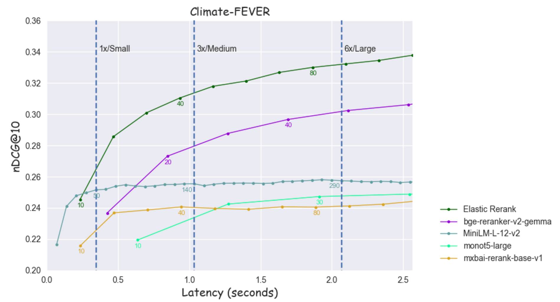
Figure 11: nDCG@10 as a function of latency for Climate-FEVER
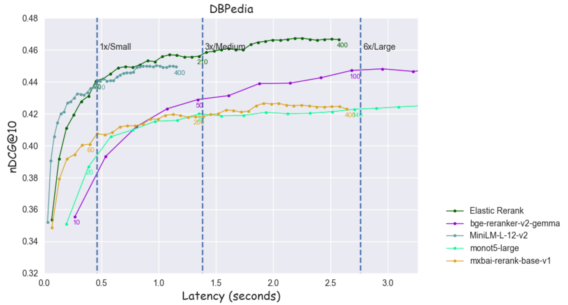
Figure 12: nDCG@10 as a function of latency for DBPedia
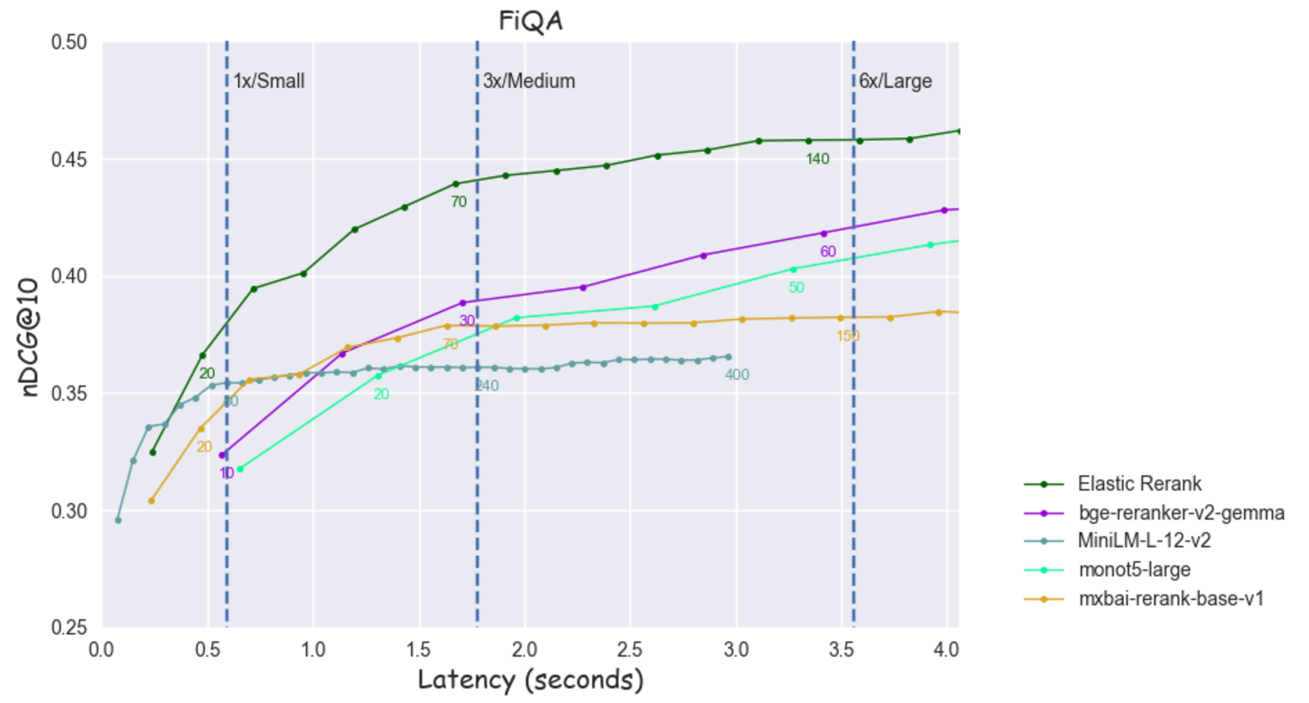
Figure 13: nDCG@10 as a function of latency for FiQA
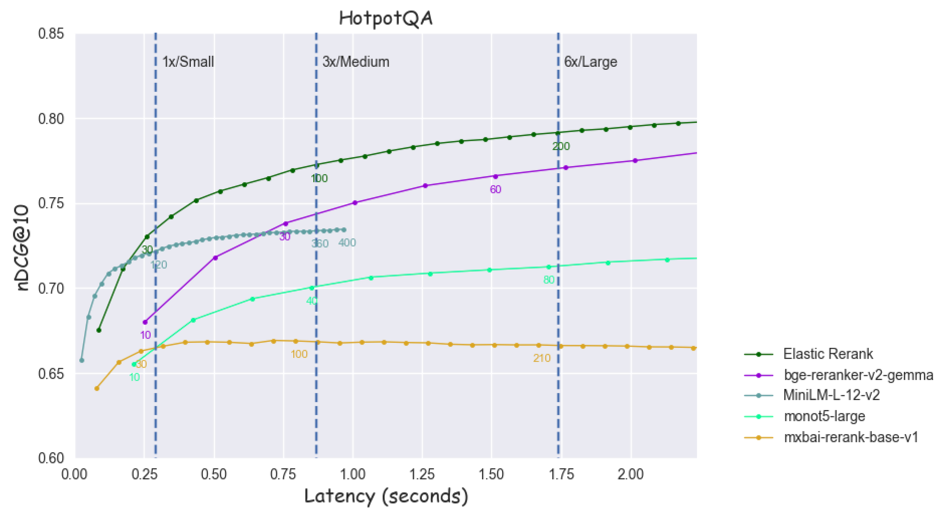
Figure 14: nDCG@10 as a function of latency for HotpotQA
Some observations:
- There are instances where the larger models are not eligible under the "Small" threshold like in the case of
bge-reranker-v2-gemmaandmonot5-largeonClimate-FEVER. MiniLM-L-12-v2provides a great example of how a smaller model can take advantage of its efficiency to "fill the gap" in terms of accuracy, especially for a low latency constraint. For example, onFiQA, under the "Small" threshold, it achieves a better score compared tobge-reranker-v2-gemmaandmxbai-rerank-base-v1even though both models are more effective eventually. This happens becauseMiniLM-L-12-v2can process many more documents (80 vs 10,20 respectively) for the same cost.- It’s common for less effective models to saturate faster which makes it feasible for "stronger" models to surpass them even when employing a small re-ranking depth. For example, on
Climate-FEVERunder the "Medium" budget thebge-reranker-v2-gemmamodel can reach a maximum depth of 20, which is enough for it to place second ahead ofMiniLM-L-12-v2andmxbai-rerank-base-v1. - The
Elastic Rerankmodel provides the optimal tradeoff between efficiency and effectiveness when considering latency values larger than a minimum threshold.
The table below presents a) the maximum permitted depth and b) the relative increase in the nDCG score (compared to BM25) for the three latency constraints applied to 5 datasets for the Elastic Rerank model.
| T-shirt size | Small | Medium | Large | |||
|---|---|---|---|---|---|---|
| Dataset | Depth | nDCG increase (%) | Depth | nDCG increase (%) | Depth | nDCG increase (%) |
| DBPedia | 70 | 37.6 | 210 | 42.43 | 400 | 45.7 |
| Climate-FEVER | 10 | 31.82 | 40 | 66.72 | 80 | 77.25 |
| FiQA | 20 | 44.42 | 70 | 73.13 | 140 | 80.49 |
| HotpotQA | 30 | 21.31 | 100 | 28.28 | 200 | 31.41 |
| Natural Questions | 30 | 70.03 | 80 | 88.25 | 180 | 95.34 |
| Average | 32 | 41.04 | 100 | 59.76 | 200 | 66.04 |
Table 5: The maximum permitted depth & associated nDCG relative increase for the Elastic Rerank model in different scenarios
We can see that a tighter budget ("Small" size scenario) allows only for the re-ranking of a few tens of documents, but that is enough to give a significant uplift (>40%) on the nDCG score.
Conclusions
In this last section we summarize the main findings and provide some guidance on how to select the optimal re-ranking depth for a given retrieval task.
Selecting a threshold
Selecting a proper re-ranking depth can have a large effect on the performance of the end-to-end system. Here, we considered some of the key dimensions that can guide this process. We were interested in approaches where a fixed threshold is applied across all queries, i.e. there is no variable-length candidate generation on a per query basis as for example in this work.
For the re-rankers we tested we found that the majority of the gain is obtained with shallow re-ranking. In particular, on average we could achieve 90% of maximum possible nDCG@10 gain re-ranking only 1/3 the number of results. For our benchmark this translated to an average re-ranking around the top 100 documents when using BM25 as a retriever. However, there is some nuance: the better the first stage retriever the fewer the candidates you need to re-rank, conversely better re-rankers benefit more from re-ranking deeper. There are also failure modes: we see effectiveness both increase to a maximum then decrease and also decrease with any re-ranking for certain models and retrieval tasks. In this context, we found more effective models are significantly less likely to ‘misbehave’ after a certain depth. There is other work that reports similar behavior.
Computational budget and non-functional requirements
We explored the impact of computational budget on re-ranking depth selection. In particular, we defined a procedure to choose the best re-ranking model and depth subject to a cost constraint. In this context, we found that the new Elastic Rerank model provided excellent effectiveness across a range of budgets for our benchmark. Furthermore, based on these experiments we’d suggest re-ranking the top 30 results from BM25 with the Elastic Rerank model when cost is at a premium. With this choice we were able to achieve around a 40% uplift in nDCG@10 on the QA portion of our benchmark.
We also have some qualitative observations:
- Re-ranking deeper with a more efficient model is often the most cost effective strategy. We found `MiniLM-L12-v2 was consistently a strong contender on a budget,
- More efficient models usually saturate faster which means that more effective models can quickly "pick-up". For example, for
DBpediaandHotpotQAElastic Rerankat depth 50 is better or on par with the performance ofMiniLM-L12-v2at depth 400.
Relevance dataset
Ideally, model and depth selection is based on relevance judgements for your own corpus. The existence of an evaluation dataset allows you to plot the evolution of retrieval metrics, such as nDCG or recall, allowing you to make an informed decision regarding the optimal threshold under desired computational cost constraints.
These datasets are usually constructed as manual annotations from domain experts or through proxy metrics based on past observations, such as Click-through Rate (CTR) on historical search results. In our previous blog we also showed how LLMs can be used to produce automated relevance judgments lists that are highly correlated with human annotations for natural language questions.
In the absence of an evaluation dataset, whatever your budget, we’d recommend starting with smaller re- ranking depths as for all the model and task combinations we evaluated this achieved the majority of the gain and also avoided some of the pathologies where quality begins to degrade. In this case you can also use the general guidelines we derived from our benchmark since it covers a broad range of retrieval tasks.
Ready to try this out on your own? Start a free trial.
Looking to build RAG into your apps? Want to try different LLMs with a vector database?
Check out our sample notebooks for LangChain, Cohere and more on Github, and join Elasticsearch Relevance Engine training now.
Related content
April 3, 2025
Generating filters and facets using ML
Exploring the pros and cons of automating the creation of filters and facets in a search experience using ML models vs the classical hard-coded approach.
February 5, 2025
Implementing clustering workflows in Elastic to enhance search relevance
We demonstrate how to integrate custom clustering models into the Elastic Stack by leveraging OpenAI text-ada-002 vectors, streamlining the workflow within Elastic’s ecosystem.

January 7, 2025
Early termination in HNSW for faster approximate KNN search
Learn how HNSW can be made faster for KNN search, using smart early termination strategies.

December 19, 2024
Understanding optimized scalar quantization
In this post, we explain a new form of scalar quantization we've developed at Elastic that achieves state-of-the-art accuracy for binary quantization.

December 10, 2024
cRank it up! - Introducing the Elastic Rerank model (in Technical Preview)
Get started in minutes with the Elastic Rerank model: powerful semantic search capabilities, with no required reindexing, provides flexibility and control over costs; high relevance, top performance, and efficiency for text search.