At Elastic we continue to work on innovations that improve the cost and performance of our vector indices. In this post we’re going to discuss in detail the implementation and intuition for a new version of scalar quantization we’ve been working on which we’re calling optimized scalar quantization or OSQ. This provides a further enhancement to our BBQ index format. Indeed, we set new state-of-the-art performance for 32 compression.
It also allows us to get very significant improvements in accuracy compared to naive scalar quantization approaches while retaining similar index compression and query performance. We plan to roll out 2, 4 and 7 bit quantization schemes and indeed unify all our index compression options to use this same underlying technique. Furthermore, we anticipate that with 7 bit quantization we should be able to discard the raw floating point vectors and plan to evaluate this thoroughly.
Measuring success
For any compression scheme we need to worry about its impact on the query behavior. For nearest neighbor queries there is a metric that much prior art focuses on. This is the recall at . Specifically, one measures the fraction of true nearest neighbor vectors that a query returns.
In fact, we already exploit the relaxation that we don't find the true nearest neighbors, even when we search with uncompressed vectors in Lucene. Linear complexity is unavoidable if one wants to find the true nearest neighbors in a high dimensional vector space. The data structure that Lucene uses to index vector data is an HNSW graph, which allows it to run approximate nearest neighbor queries significantly faster than a linear scan.
In this blog we study a metric that we’ll abbreviate as recall@, which is the recall at retrieving candidates and reranking them using the uncompressed vector distance calculation. Note that if then it's simply equal to the recall at . We also look at the quality of the approximation of the uncompressed vector distances.
We’ll discuss all this in more detail when we discuss our results.
Motivation
Scalar quantization, as we’ve discussed before, is an approach which allows one to represent floating point vectors by integer vectors. There are two reasons to do this:
- It allows you to reduce the amount of memory needed to represent a vector, by using fewer than 32 bits per integer, and
- It allows you to accelerate the distance calculation between vectors, which is the bottleneck for performing nearest neighbor queries in vector databases.
Recently, a paper, which we’ve discussed before, proposed an approach called RaBitQ that is able to achieve good recall using only 1 bit per component. This is exciting because 32 compression is competitive with Product Quantization (PQ), which was the previous state-of-the-art approach when compression was paramount. A key advantage of RaBitQ is that it’s relatively straightforward to accelerate distance calculations with SIMD operations. Certainly, when it is compared to PQ that uses lookups to compute distance, for which it is much harder to exploit hardware parallelism. The authors performed extensive experiments and showed they were able to achieve consistently higher recall as a function of query latency than PQ using the same compression ratio with an IVF index.
Although the RaBitQ approach is conceptually rather different to scalar quantization, we were inspired to re-evaluate whether similar performance could be unlocked for scalar quantization. In our companion piece we will discuss the result of integrating OSQ with HNSW and specifically how it compares to the baseline BBQ quantization scheme, which is inspired by RaBitQ. As an incentive to keep reading this blog we note that we were able to achieve systematically higher recall in this setting, sometimes by as much as 30%. Another advantage of OSQ is it immediately generalizes to using bits per component. For example, we show below that we’re able to achieve excellent recall in all cases we tested using minimal or even no reranking with only a few bits per component.
This post is somewhat involved. We will take you through step-by-step the innovations we’ve introduced and explain some of the intuition at each step.
Dot products are enough
In the following we discuss only the dot product, which would translate to a MIP query in Elasticsearch. In fact, this is sufficient because well known reductions exist to convert the other metrics Elasticsearch supports, Euclidean and cosine, to computing a dot product. For the Euclidean distance we note that
and also that and can be precomputed and cached, so we need only compute the dot product in order to compare two vectors. For cosine we simply need to normalize vectors and then
Scalar quantization refresher
Scalar quantization is typically defined by the follow componentwise equation
Here, . The quantized vector is integer valued with values less than or equal to , that is we’re using bits to represent each component. The interval is called the quantization interval.
We also define the quantized approximation of the original floating point vector, which is our best estimate of the floating point vector after we’ve applied quantization. We never directly work with this quantity, but it is convenient to describe the overall approach. This is defined as follows
Here, denotes a vector whose components are all equal to one. Note that we abuse notation here and below by using to denote both a vector and scalar and we rely on the context to make the meaning clear.
The need for speed
A key requirement we identified for scalar quantization is that we can perform distance comparisons directly on integer vectors. Integer arithmetic operations are more compute efficient than floating point ones. Furthermore, higher throughput specialized hardware instructions exist for performing them in parallel. We’ve discussed how to achieve this in the context of scalar quantization before.
Below we show that as long as we cache a couple of corrective factors we can use a different quantization interval and number of bits for each vector we quantize and still compute the dot product using integer vectors. This is the initial step towards achieving OSQ.
First of all observe that our best estimate of the dot product between two quantized vectors is
Expanding we obtain
Focusing on the vector dot products, since these dominate the compute cost, we observe that is just equal to the vector dimension, and and are the sums of the quantized query and document vector components, respectively. For the query this can be computed once upfront and for the documents these can be computed at index time and stored with the quantized vector. Therefore, we need only compute the integer vector dot product per comparison.
The geometry of scalar quantization
To build a bit more intuition about OSQ we digress to understand more about how scalar quantization represents a vector. Observe that the set of all possible quantized vectors lie inside a cube centered on the point with side length . If only 1 bit is being used then the possible vectors lie at the corners of the cube. Otherwise, the possible vectors lie on a regular grid with points.
By changing and , we are only able to expand or contract the cube or slide it along the line spanned by the vector. In particular, suppose the vectors in the corpus are centered around some point . We can decompose this into a component parallel to the vector and a component perpendicular to it as follows
If we center the cube on the point at then it must still expand it to encompass the offset before it covers even the center of the data distribution. This is illustrated in the figure below for 2 dimensions.
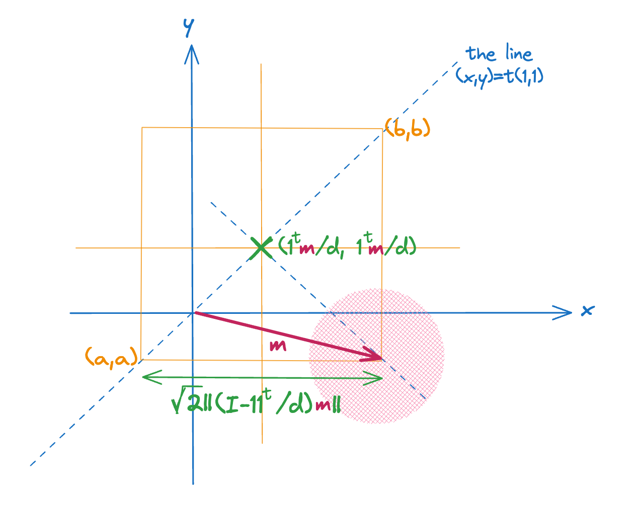
Since the quantization errors will be proportional on average to the side length of the cube, this suggests that we want to minimize . An easy way to do this is to center the query and document vectors before quantizing. We show below that if we do this we can still recover the dot product between the original vectors.
Note that
The values and , which are the inner product between the query and document vector and the centroid of the vectors in the corpus, can be precomputed and in the case of the document vector cached with its quantized representation. The quantity is a global constant.
This means we only need to estimate when comparing a query and document vector. In other words, we can quantize the centered vectors and recover an estimate of the actual dot product.
The distribution of centered vectors
So far we’ve shown that we can use a different bit count and a different quantization interval per vector. We next show how to exploit this to significantly improve the accuracy of scalar quantization. We propose an effective criterion and procedure for optimizing the choice of the constants and . However, before discussing this it is useful to see some examples of the component distribution in real centered embedding vectors.
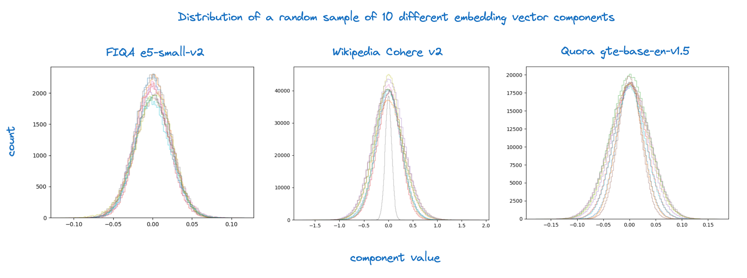
We observe that the values are all fairly normally distributed and will use this observation to choose our initial quantization interval.
Looking at these plots one might guess it would be beneficial to scale components. Specifically, it seems natural to standardize the component distributions of the Cohere v2 and the gte-base-en-v1.5 embeddings. In general, this would amount to applying a scaling matrix to the document vectors before quantization as follows
Here, is a diagonal matrix whose diagonal entries are the standard deviations of the components for the corpus as a whole. We can apply this operation and still compute the dot product efficiently because we simply need to apply the inverse transformation to the query vector before quantizing it
The effect is not symmetric because, as we’ll discuss below, we use a higher bit count for the query.
Referring back to our geometric picture this would amount to stretching the different edges of the cube. We tried this but found it didn’t measurably improve effectiveness once we optimize the interval directly for each vector so avoid the extra complexity.
Initializing the quantization interval
Let’s consider a natural criterion for setting a global quantization interval for normally distributed data. If we pick a vector, , at random from the corpus then the quantization error is given by
By assumption, and as we showed empirically is often the case, each component of is normally distributed or . In such a scenario it is reasonable to minimize the expected square error. Specifically, we seek
Since the expectation is a linear operator it distributes over the summation and we can focus on a single term. Without loss of generality we can assume that is a unit normal since we can always rescale the interval by the data standard deviation.
To compute this expectation we make use of the following quantity
This is the expectation of the square error when rounding a normally distributed value to a fixed point expressed as an indefinite integral, alternatively, before we’ve determined the range the value can take.
In order to minimize the expected quantization error we should snap floating point values to their nearest grid point. This means we can express the expected square quantization error as follows
Where we defined . The integration limits are determined by the condition that we snap to the nearest grid point.
We now have a function, in terms of the interval endpoints and , for the expected square quantization error using a reasonable assumption about the vector components’ distribution. It is relatively straightforward to show that this quantity is minimized by an interval centered on the origin. This means that we need to search for the value of a single variable which minimizes . The figure below shows the error as a function of for various bit counts.
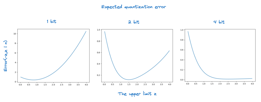
Optimizing this function numerically for various choices of gives the following quantization intervals
We’re denoting the interval for bits .
Finally, we need to map these fixed intervals to the specific interval to use for a vector . To do this we shift by the mean of its components and scale by their standard deviation . It’s clear that we should always choose and . Therefore, our initial estimate for the quantization interval for a vector using bits per component is
Refining the quantization interval
The initialization scheme actually works surprisingly well. We present the results of quantizing using this approach alone as one of the ablation studies when we examine the performance of OSQ. However, we can do better.
It has been noted in the context of PQ that targeting minimum square quantization error is not actually the best criterion when you care about recall. In particular, you know you’re going to be running nearest neighbor queries on the corpus and the nearest neighbors of a query are very likely to be fairly parallel to the query vector. Let’s consider what this means.
Suppose we have query vector for which the document is relevant. Ignoring the quantization of the query vector, we can decompose the square of the error in the dot product into a component that is parallel to and a component which is perpendicular to the document vector as follows
Now we expect . Furthermore, we would like to minimize the error in the dot product in this specific case, since this is when the document is relevant and our query should return it.
Let for some . We can bound our quantization error in the dot product as follows
Whatever way we quantize we can’t affect the quantity so all we care about is minimizing the second factor. A little linear algebra shows that this is equal to
Here, we’ve made the dependence of this expression on the quantization interval explicit.
So far we’ve proposed a natural quantity to minimize in order to reduce the impact of quantization on MIP recall. We now turn our attention to how to efficiently minimize this quantity with respect to the interval .
There is a complication because the assignment of components of the vector to grid points depends on and while the optimal choice for and depends on this assignment. We use a coordinate descent approach, which alternates between computing the quantized vector while holding and fixed, and optimizing the quantization interval while holding fixed. This is described schematically as follows.
1
2 for do
3 compute from and
4
5 if then break
First we’ll focus on line 3. The simplest approach to compute uses standard scalar quantization
Specifically, this would amount to snapping each component of to the nearest grid point. In practice this does not minimize as we illustrate below.
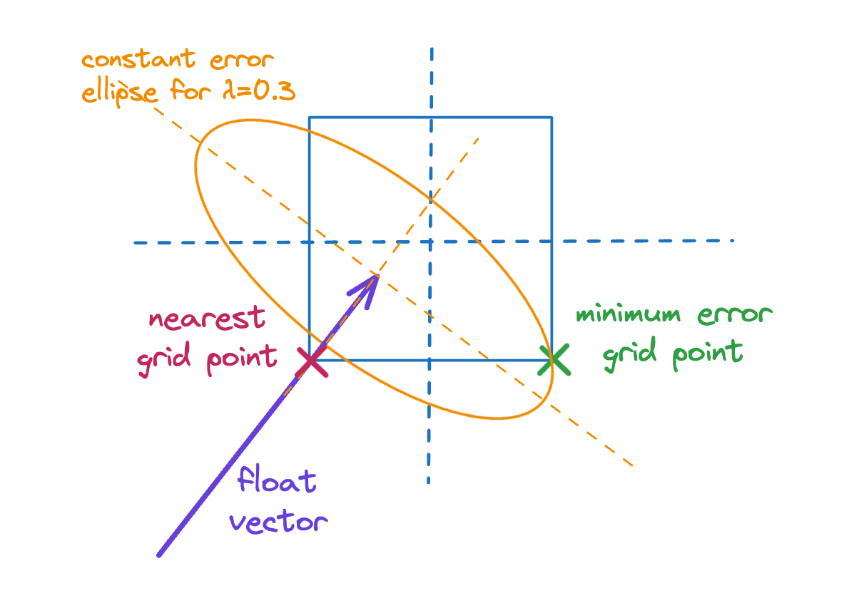
Unfortunately, we can’t just enumerate grid points and find the minimum error one since there are candidates; therefore, we tried the following heuristic:
- Snap to the nearest grid point,
- Coordinate-wise check if rounding in the other direction reduces the error.
This isn’t guaranteed to find the global optimum, which in fact isn’t guaranteed to be one of the corners of the grid square containing the floating point vector. However, in practice we found it meant the error almost never increased in an iteration of the loop over . By contrast, when snapping to the nearest grid point the loop frequently exits due to this condition.
The heuristic yields a small but systematic improvement in the brute force recall. On average it amounted to +0.3% compared to just snapping to the nearest grid point. Given the impact is so small we decided it wasn’t worth the extra complexity and increased runtime.
We now turn our attention to line 4. This expression decomposes as follows
It’s fairly easy to see that this is a convex quadratic form of and . This means it has a unique minimum where the partial derivatives w.r.t. and vanish. We won’t show the full calculation but give a flavor. For example, we can use the chain rule to help evaluate the first term
then
Where we’ve defined . The final result is that the optimal interval satisfies
which is trivial to solve for and . Taken together with the preprocessing and interval initialization steps this defines OSQ.
The query and document vectors are different
We noted already that each vector could choose its bit count. Whilst there are certain technical disadvantages to using different bit counts for different document vectors, the query and the document vectors are different. In particular, the compression factor the quantization scheme yields only depends on the number of bits used to represent the document vectors.
There are side effects from using more bits to represent the query, principally that it can affect the dot product performance. Also there’s a limit to what one can gain based on the document quantization error. However, we get large recall gains by using asymmetric quantization for high compression factors and this translates to significant net wins in terms of recall as a function of query latency. Therefore, we always quantize the query using at least 4 bits.
How does it perform?
In this section we compare the brute force recall@ and the correlation between the estimated and actual dot products for OSQ and our baseline BBQ quantization scheme, which was an adaptation of RaBitQ to use with an HNSW index. We have previously evaluated this baseline scheme and its accuracy is commensurate with RaBitQ. The authors of RaBitQ did extensive comparisons with alternative methods showing its superiority; we therefore consider it sufficient to simply compare to this very strong baseline.
We also perform a couple of ablation studies: against a global interval and against the per vector intervals calculated by our initialization scheme. To compute a global interval we use the OSQ initialization strategy, but compute the mean and variance of the corpus as a whole. For low bit counts, this is significantly better than the usual fixed interval quantization scheme, which tends to use something like the 99th percentile centered confidence interval. High confidence intervals in such cases often completely fail because the grid points are far from the majority of the data.
We evaluate against a variety of embeddings
and datasets
- Quora
- FiQA
- A sample of around 1M passages from the English portion of wikipedia-22-12
- GIST1M
The embedding dimensions vary from 384 to 960. E5, Arctic and GTE use cosine similarity, and Cohere and GIST using MIP. The datasets vary from around 100k to 1M vectors.
In all our experiments we set , which we found to be an effective choice.
First off we study 1 bit quantization. We report brute force recall in these experiments to take any effects of the indexing choice out of the picture. As such we do not compare recall vs latency curves, which are very strongly affected by both the indexing data structure and the dot product implementation. Instead we focus on the recall at 10 reranking the top n hits. In our next blog we’ll study how OSQ behaves when it is integrated with Lucene's HNSW index implementation and turn our attention to query latency. The figures below show our brute force recall@ for .
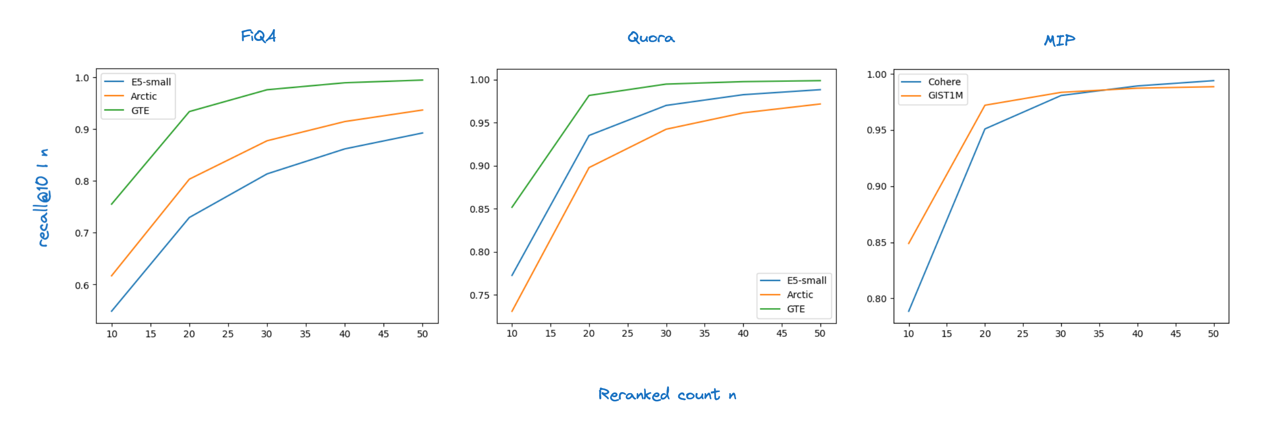
Rolling these up into the average recall@ for the 8 retrieval experiments we tested we get the table below.
| n | Baseline average recall@10|n | OSQ average recall@10|n | Global average recall@10|n | Initialization average recall@10|n |
|---|---|---|---|---|
| 10 | 0.71 | 0.74 | 0.54 | 0.65 |
| 20 | 0.88 | 0.90 | 0.69 | 0.81 |
| 30 | 0.93 | 0.94 | 0.76 | 0.86 |
| 40 | 0.95 | 0.96 | 0.80 | 0.89 |
| 50 | 0.96 | 0.97 | 0.82 | 0.90 |
Compared to the baseline we gain 2% on average in recall. As for the ablation study, compared to using a global quantization interval we gain 26% and compared to our initial per vector quantization intervals we gain 10%.
The figure below shows the floating point dot product values versus the corresponding 1 bit quantized dot product values for a sample of 2000 gte-base-en-v1.5 embeddings. Visually the correlation is high.
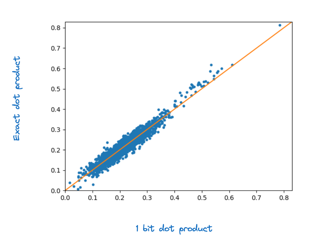
We can quantify this by computing the between the floating point and quantized dot products. For each dataset and model combination we computed the average for every query against the full corpus. We see small but systematic improvement in comparing OSQ to the baseline. The table below shows the values broken down by the dataset and model combinations we tested.
| Dataset | Model | Baseline R2 | OSQ R2 |
|---|---|---|---|
| FiQA | e5-small | 0.849 | 0.865 |
| FiQA | arctic | 0.850 | 0.863 |
| FiQA | gte | 0.925 | 0.930 |
| Quora | e5-small | 0.868 | 0.881 |
| Quora | arctic | 0.817 | 0.838 |
| Quora | gte | 0.887 | 0.897 |
| Wiki | Cohere v2 | 0.884 | 0.898 |
| GIST1M | - | 0.953 | 0.974 |
Interestingly, when we integrated OSQ with HNSW we got substantially larger improvements in recall than we see for brute force search, as we’ll show in our next blog. One hypothesis we have is that the improvements we see in correlation with the true floating point dot products are more beneficial for graph search than brute force search. For many queries the tail of high scoring documents are well separated from the bulk of the score distribution and are less prone to being reordered by quantization errors. By contrast we have to navigate through regions of low scoring documents as we traverse the HNSW graph. Here any gains in accuracy can be important.
Finally, the table below compares the average recall for 1 and 2 bit OSQ for the same 8 retrieval experiments. With 2 bits we reach 95% recall reranking between 10 and 20 candidates. The average rises from 0.893 for 1 bit to 0.968 for 2 bit.
| n | 1 bit OSQ average recall@10|n | 2 bit OSQ average recall@10|n |
|---|---|---|
| 10 | 0.74 | 0.84 |
| 20 | 0.90 | 0.97 |
| 30 | 0.94 | 0.99 |
| 40 | 0.96 | 0.995 |
| 50 | 0.97 | 0.997 |
Conclusion
We’ve presented an improved automatic scalar quantization scheme which allows us to achieve high recall with relatively modest reranking depth. Avoiding deep reranking has significant system advantages.
For 1 bit quantization we compared it to a very strong baseline and showed it was able to achieve systematic improvements in both recall and the accuracy with which it approximates the floating point vector distance calculation. Therefore, we feel comfortable saying that it sets new state-of-the-art performance for at 32 compression of the raw vectors.
It also allows one to simply trade compression for retrieval quality using the same underlying approach and achieves significant performance improvements compared to standard scalar quantization techniques.
We are working on integrating this new approach into Elasticsearch. In our next blog we will discuss how it is able to enhance the performance of our existing BBQ scalar quantization index formats.
Ready to try this out on your own? Start a free trial.
Looking to build RAG into your apps? Want to try different LLMs with a vector database?
Check out our sample notebooks for LangChain, Cohere and more on Github, and join Elasticsearch Relevance Engine training now.
Related content

December 4, 2024
Smokin' fast BBQ with hardware accelerated SIMD instructions
How we optimized vector comparisons in BBQ with hardware accelerated SIMD (Single Instruction Multiple Data) instructions.
November 11, 2024
Better Binary Quantization (BBQ) in Lucene and Elasticsearch
How Better Binary Quantization (BBQ) works in Lucene and Elasticsearch.

October 22, 2024
RaBitQ binary quantization 101
Understand the most critical components of RaBitQ binary quantization, how it works and its benefits. This guide also covers the math behind the quantization and examples.
November 18, 2024
Better Binary Quantization (BBQ) vs. Product Quantization
Why we chose to spend time working on Better Binary Quantization (BBQ) instead of product quantization in Lucene and Elasticsearch.

November 11, 2023
Understanding scalar quantization in Lucene
Explore how Elastic introduced scalar quantization into Lucene, including automatic byte quantization, quantization per segment & performance insights.