Today, users have come to expect search results that are tailored to their individual interests. If all the songs we listen to are rock songs, we would expect an Aerosmith song at the top of the results when searching for Crazy, not the one by Gnarls Barkley. In this article, we take a look at ways to personalize search before diving into the specifics of how to do this with learning-to-rank (LTR), using music preferences as an example.
Ranking factors
First, let's recap which factors are important in search ranking in general. Given a user query, a relevance function can take into account one or multiple of the following factors:
- Text similarity can be measured with a variety of methods including BM25, dense vector similarity, sparse vector similarity or through cross-encoder models. We can calculate similarity scores of the query string against multiple fields in a document (title, description, tags, etc.) to determine how well the input query matches a document.
- Query properties can be inferred from the query itself, for example the language, named entities or the user intent. The domain will influence which of these properties can be most helpful to improve relevance..
- Document properties pertain to the document itself, for example its popularity or the price of the product represented by the document. These properties often have a big impact on the relevance when applied with the right weights.
- User and context properties refer to data that is not associated with the query or the document but with the context of the search request, for example the location of the user, past search behavior or user preferences. These are the signals that will help us personalize our search.

Personalized results
When looking at the last category of factors, user and context properties, we can distinguish between three types of systems:
- "General" search does not take into account any user properties. Only query input and document properties determine the relevance of search results. Two users that enter the same query see the same results. When you start Elasticsearch you have such a system out-of-the-box.
- Personalized search adds user properties to the mix. The input query is still important but it is now supplemented by user and/or context properties. In this setting users can get different results for the same query and hopefully the results are more relevant for individuals.
- Recommendations goes a step further and focuses exclusively on document, user and context properties. There is no actively supplied user query to these systems. Many platforms recommend content on the home page that is tailored to the user’s account, for example based on the shopping history or previously watched movies.
If we look at personalization as a spectrum, personalized search sits in the middle. Both user input and user preferences are part of the relevance equation. This also means that personalization in search should be applied carefully. If we put too much weight on past user behavior and too little on the present search intent, we risk frustrating users with their favorite documents when they were specifically searching for something else. Maybe you too had the experience of watching that one folk dance video that your friend posted and subsequently found more of these when searching for dance music. The lesson here is that it's important to ensure sufficient amounts of historic data for a user in order to confidently skew search results in a certain direction. Also keep in mind that personalization is mainly going to make a difference for ambiguous user input and exploratory queries. Unambiguous navigational queries should already be covered by your general search mechanisms.
There are many methods for personalization. There are rule-based heuristics in which developers hand-craft the matching of user properties onto sets of specific documents, for example manually boosting onboarding documents for new users. There are also low tech methods of sampling results from general and personal result lists. Many of the more principled approaches use vector representations trained either on item similarity or with collaborative filtering techniques (e.g. “customers also bought”). You can find many posts around these methods online. In this post we will focus on using learning-to-rank.
Personalized search with LTR
Learning-to-rank (LTR) is the process of creating statistical models for relevance ranking. You can think of it as automatically tuning the weights of different relevance factors. Instead of manually coming up with a structured query and weights for all text similarity, query properties and document properties, we train a model that finds an optimal trade-off given some data. The data comes in the form of a judgment list. Here we are going to look at behavior-based personalization using LTR, meaning that we will utilize past user behavior to extract user properties that will be used in our LTR training process.
It's important to note that, in order to set yourself up for success, you should be already well underway in your LTR journey before you start with personalization:
- You should already have LTR in place. If you want to introduce LTR into your search, it's best to start by optimizing your general (non-personalized) search first. There might be some low-hanging fruit there and this will give you the chance to build a solid technical base before adding complexity. Dealing with user-dependent data means you need more of it during training and evaluation becomes trickier. We recommend waiting with personalization until your overall LTR setup is in a solid state.
- You should already be collecting usage data. Without it you would not have enough data for sensical improvements to your relevance: the cold start problem. It's also important that you have high confidence in the correctness of your usage tracking data. Incorrectly sent tracking events and erroneous data pipelines can often go undetected because they don’t throw any errors, but the resulting data ends up misrepresenting the actual user behavior. Subsequently basing personalization projects on this data will probably not succeed.
- You should already be creating your judgment list from usage data. This process is also known as click modeling and it is both a science and an art. Here, instead of manually labeling relevant and irrelevant documents in search results, you use click signals (clicks on search results, add-to-cart, purchases, listening to a whole song, etc.) to estimate the relevance of a document that a user was served as part of past search results. You probably need multiple experiments to get this right. Plus, there are some biases that are being introduced here (most notably position bias). You should feel confident that your judgment list well represents the relevance for your search.

If all these things are a given, then let's go ahead and add personalization. First, we are going to dive into feature engineering.
Feature engineering
In feature engineering we ask ourselves which concrete user properties can be used in your specific search to make results more relevant? And how can we encode these properties as ranking features? You should be able to imagine exactly how adding, say, the location of the user could improve the result quality. For instance code search is typically a use case that is independent of the user location. Music tastes on the other hand are influenced by local trends. If we know where the searcher is and we know to which geo location we can attribute a document, this can work out. It pays to be thoughtful about which user features and which document feature might work together. If you cannot imagine how this would work in theory, it might not be worth adding a new feature to your model. At any rate, you should always test the effectiveness of new features both offline after training and later in an online A/B test.
Some properties can be directly collected from the tracking data, such as the location of the user or the upload location of a document. When it comes to representing user preferences, we have to do some more calculations (as we will see below). Furthermore we have to think about how to encode our properties as features because all features must be numeric. For example, we have to decide whether to represent categorical features as labels represented by integers or as one-hot encoding of multiple binary labels.
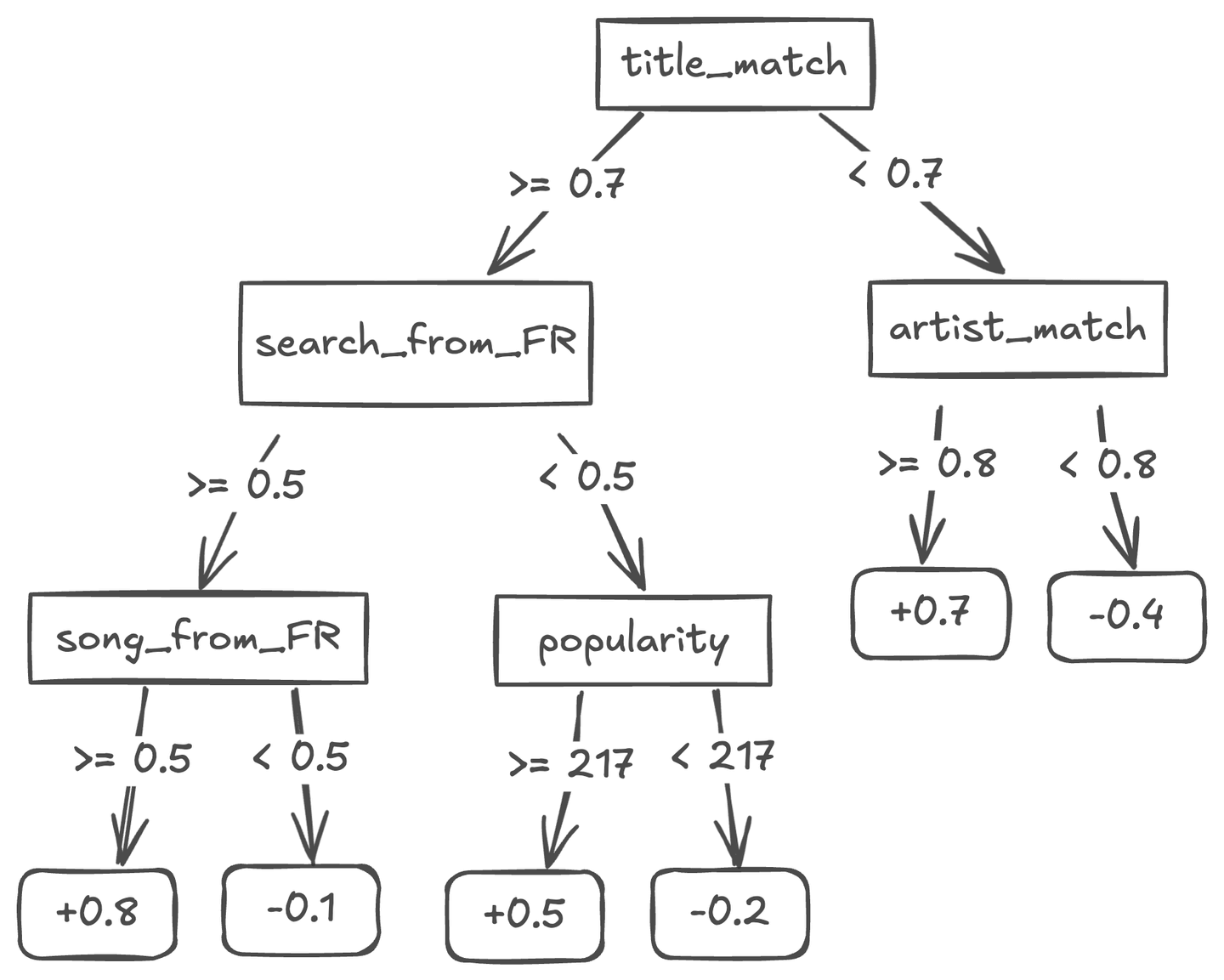
To illustrate how user features might influence relevance ranking, consider the fictive example boosting tree below that could be part of an XGBoost model for a music search engine. The training process learned the importance of the location feature "from France" (on the left-hand side) and weighed them against the other features such as text similarity and document features. Note that these trees are typically much deeper and there are many more of them. We chose a one-hot encoding for the location feature both on the search and on the documents.

Be aware that the more features are added, the more nodes in these trees are required to make use of them. Consequently more time and resources will be needed during training in order to reach convergence. Start small, measure improvements and expand step-by-step.
Example of personalized search with LTR: music preferences
How can we implement this in Elasticsearch? Let's again assume we have a search engine for a music website where users can look for songs and listen to them. Each song is categorized into a high-level genre. An example document could look like this:
{
  "title": "Personal Jesus",
  "artist": "Depeche Mode",
  "genre": "pop"
}
Further assume that we have an established way to extract a judgment list from usage data. Here we use relevance grades from 0 to 3 as an example, which could be computed from no interaction, clicking on a result, listening to the song and giving a thumbs-up rating for the song. Doing this introduces some biases in our data, including position bias (more on this in a future post). The judgment list could look like this:
query_id  query   user_id  document_id  grade
q:1       jump    u:1      d:1          1
q:1       jump    u:1      d:2          3
q:1       jump    u:1      d:3          0
q:2       crazy   u:2      d:4          2
q:2       crazy   u:2      d:5          0
We track the songs that users listen to on our site, so we can build a dataset of music genre preferences for each user. For example, we could look back some time into the past and aggregate all genres that a user has listened to. Here we could experiment with different representations of genre preferences, including latent features, but for simplicity we'll stick to relative frequencies of listens. In this example we want to personalize for individual users but note that we could also base our calculations on segments of users (and use segment IDs).
user_id  user_hiphop  user_pop  user_rock
u:1      0.2          0.7       0.1
u:2      0.4          0.2       0.4
u:3      0.8          0.0       0.2
When calculating this, it would be wise to take the amount of activity of users into account. This goes back to the folk dance example above. If a user only interacted with one song, the genre preference would be completely skewed to its genre. To prevent the subsequent personalization putting too much weight on this, we could add the number of interactions as a feature so the model can learn when to put weight on the genre plays. We could also smooth the interactions and add a constant to all frequencies before normalizing so they don’t deviate from a uniform distribution for low counts. Here we assume the latter.
The above data needs to be stored in a feature store so that we can look up the user preference values by user ID both during training and at search time. You can use a dedicated Elasticsearch index here, for example:
PUT genre-preferences/_doc/u:1
{
  "user_hiphop": 0,2,
  "user_pop": 0.7,
  "user_rock": 0.1
}
With the user ID as the Elasticsearch document ID we can use the Get API (see below) to retrieve the preference values. This will have to be done in your application code as of Elasticsearch version 8.15. Also note that these separately stored feature values will need to be refreshed by a regularly running job in order to keep the values up-to-date as preferences change over time.
Now we are ready to define our feature extraction. Here we one-hot-encode the genres. We plan to also enable representing categories as integers in future releases.
from eland.ml.ltr import LTRModelConfig, QueryFeatureExtractor

feature_extractors = [
    # Example text similarity feature
    QueryFeatureExtractor(
        feature_name="title_match",
        query={"match": {"title": "{{query}}"}},
    ),

    # One-hot encode genre categories. Make sure `genre` is of type `keyword`.
    QueryFeatureExtractor(
        feature_name="is_hiphop",
        query={
            "constant_score": {
                "filter": { "term": { "genre": "hiphop" } },
                "boost": 1,
            }
        },
    ),
    QueryFeatureExtractor(
        feature_name="is_pop",
        query={
            "constant_score": {
                "filter": { "term": { "genre": "pop" } },
                "boost": 1,
            }
        },
    ),
    QueryFeatureExtractor(
        feature_name="is_rock",
        query={
            "constant_score": {
                "filter": { "term": { "genre": "rock" } },
                "boost": 1,
            }
        },
    ),

    # Forward user preference values from the params as features
    QueryFeatureExtractor(
        feature_name="user_hiphop",
        query={
            "query": {"match_all": {}},
            "script_score": {"script": {"source": "{{user_hiphop}}"} },
        },
    ),
    QueryFeatureExtractor(
        feature_name="user_pop",
        query={
            "query": {"match_all": {}},
            "script_score": {"script": {"source": "{{user_pop}}"} },
        },
    ),
    QueryFeatureExtractor(
        feature_name="user_rock",
        query={
            "query": {"match_all": {}},
            "script_score": {"script": {"source": "{{user_rock}}"} },
        },
    ),
]

ltr_config = LTRModelConfig(feature_extractors)
Now when applying the feature extraction, we have to first look up the genre preference values and forward them to the feature logger. Depending on performance, it might be good to batch lookup these values.
import numpy as np

PREFERENCES_INDEX = "genre-preferences"

def get_genre_preferences(es_client, index_name, user_id):
    return es_client.get(index=index_name, id=user_id)["_source"]

def extract_query_features(query_group):
    # get query string, user ID and document IDs from the judgment list
    query_string = query_group["query"].iloc[0]
    user_id = query_group["query"].iloc[0]
    doc_ids = query_group["doc_id"].astype("str").to_list()

    # get genre preference values from Elasticsearch index
    # (consider using mget outside this function in case of slowness)
    genre_preferences = get_genre_preferences(es_client, PREFERENCES_INDEX, user_id)

    # run the extraction
    search_params = {
        "query": query_string,
        "user_hiphop": genre_preferences["user_hiphop"],
        "user_pop": genre_preferences["user_pop"],
        "user_rock": genre_preferences["user_rock"],
    }
    features = feature_logger.extract_features(search_params, doc_ids)

    # add features as new columns
    for feature_index, feature_name in enumerate(ltr_config.feature_names):
        query_group[feature_name] = np.array(
            [doc_features[doc_id][feature_index] for doc_id in doc_ids]
        )

    return query_group


# extract features for all data with the same query ID
judgments_df.groupby("query_id", group_keys=False).apply(_extract_query_features)
After feature extraction, we have our data ready for training. Please refer to the previous LTR post and the accompanying notebook for how to train and deploy the model (and make sure to not send the IDs as features).
query_id  query   user_id  document_id  grade  title_match  is_hiphop  is_pop  is_rock  user_hiphop  user_pop  user_rock
q:1       jump    u:1      d:1          1      1.4          1          0       0        0.2          0.7       0.1
q:1       jump    u:1      d:2          3      1.4          0          0       1        0.2          0.7       0.1
q:1       jump    u:1      d:3          0      1.2          0          1       0        0.2          0.7       0.1
q:2       crazy   u:2      d:4          2      2.2          0          0       1        0.4          0.2       0.4
q:2       crazy   u:2      d:5          0      2.2          0          0       0        0.4          0.2       0.4
Once the model is trained and deployed, you can use it in a rescorer like this. Note that at search time you also need to look up the user preference values beforehand and add the values to the query.
# inputs
user_query = "crazy"
user_id = "u:42"

# preference lookup
genre_preferences = get_genre_preferences(es_client, PREFERENCES_INDEX, user_id)

# search
query = {
  "match": {
    "title": user_query
  }
}

rescore = {
  "learning_to_rank": {
    "model_id": "my-genre-personalization-model",
    "params": {
      "query": user_query,
      "user_hiphop": genre_preferences["user_hiphop"],
      "user_pop": genre_preferences["user_pop"],
      "user_rock": genre_preferences["user_rock"]
    }
  },
  "window_size": 100
}

es_client.search(index="my-music-index", query=query, rescore=rescore)
Now the users of our music website with different genre preferences can benefit from your personalized search. Both rock and pop lovers will find their favorite version of the song called Crazy at the top of the search results.
Conclusion
Adding personalization has the potential to improve relevance. One way to personalize search is through LTR in Elasticsearch. We have looked at some prerequisites that should be given and went through a hands-on example.
However, in the name of a focused post, we left out several important details. How would we evaluate the model? There are offline metrics that can be applied during model development, but ultimately an online A/B test with real users will have to decide if the model improves relevance. How do we know if we are using enough data? Spending more resources at this stage can improve quality but we need to know under which conditions this is worth it. How would we build a good judgment list and deal with the different biases introduced by using behavioral tracking data? And can we forget about our personalized model after deployment or do we require repeated maintenance to address drift? Some of these questions will be answered in future posts on LTR, so stay tuned.
Ready to try this out on your own? Start a free trial.
Want to get Elastic certified? Find out when the next Elasticsearch Engineer training is running!
Related content

September 15, 2025
Balancing the scales: Making reciprocal rank fusion (RRF) smarter with weights
Exploring weighted reciprocal rank fusion (RRF) in Elasticsearch and how it works through practical examples.

September 8, 2025
MCP for intelligent search
Building an intelligent search system by integrating Elastic's intelligent query layer with MCP to enhance the generative efficacy of LLMs.

Building intelligent duplicate detection with Elasticsearch and AI
Explore how organizations can leverage Elasticsearch to detect and handle duplicates in loan or insurance applications.

July 10, 2025
Diversifying search results with Maximum Marginal Relevance
Implementing the Maximum Marginal Relevance (MMR) algorithm with Elasticsearch and Python. This blog includes code examples for vector search reranking.

July 9, 2025
Semantic text is all that and a bag of (BBQ) chips! With configurable chunking settings and index options
Semantic text search is now customizable, with support for customizable chunking settings and index options to customize vector quantization, making semantic_text more powerful for expert use cases.