Introduction
In a typical search scenario, tools like BM25, ELSER, and re-rankers assign scores to documents based on how well they match a given query. These scores help rank the documents, but they don't always translate easily into clear, concrete relevance levels. That’s where calibration comes in—it either forces a model to produce scores on a fixed, understandable scale or connects the existing scores to a defined relevance level. This step is crucial for improving the transparency and explainability of a search process and filtering out irrelevant results so users aren’t shown unhelpful content.
It’s worth noting that some algorithms, such as BM25, have score scales that vary between queries due to their dependence on query terms. This can make calibration challenging to implement. However, with NLP-based retrievers and re-rankers, it’s a bit easier because their scoring is usually more consistent across queries. In this post, we’ll explore how to calibrate an NLP model’s scoring system by attaching a relevance scale to it. This approach makes search results more understandable and useful for both developers and users.
To achieve this, you'll need an annotated dataset of a few thousand pairs (we will discuss this later in the blog). The guidelines for annotation play a key role in defining a good relevance scale. This scale can be simple, like a binary system (a document is either relevant or irrelevant), or more nuanced, with multiple levels (e.g. 0: irrelevant, 1: related but unhelpful, 2: helpful but incomplete, 3: perfect match). The annotation process itself is critical but often costly, especially when it's done by humans.
While we won’t dive into it here, recent advances in large language models (LLMs) have made automating this process much easier and more affordable, with humans only needing to verify the results. We'll cover this in future posts. For now, let's assume you already have an annotated dataset and focus on understanding how to interpret a model’s scoring system.
Class balanced expected calibration error
Before looking at actual code and the steps needed to calibrate our scores, it might be helpful to introduce core concepts that will help us build our calibration tools. One notion of miscalibration is the difference in expectation between confidence and accuracy. Expected Calibration Error is trying to calculate that by partitioning predicted scores into M equally spaced bins (similar to reliability diagrams) and taking a weighted average of the bins' accuracy and confidence difference:
where is the total number of samples and the number of samples in bin . The accuracy and the confidence within a bin can be defined as:
where , are predicted and true class label for the sample and represents the confidence that the sample is relevant to a given query. Note that this definition works for binary classification. In the case you have multiple labels and an unbalanced annotated dataset, which is not uncommon, you need to introduce a revised definition. This is where Class Balanced - ECE becomes useful. We first split our dataset into subsets where when . Here, is the score of sample i for a given query. Then we have:
This time, accuracy and confidence are defined as:
We then calculate the final calibration score by taking the weighted average of all values. The underlying hypothesis is that, with an imbalanced dataset, a sufficiently accurate predictor each will contain a different number of samples. So by treating them equally when averaging, we aim to prevent any bias toward a specific class. Another key requirement is that model scores align with the range of label scores to enable accurate bin construction. This can be achieved using a simple min-max scaling transformation on scores to the label range.
This metric reflects only how aligned and linear your scoring space is. While it can be helpful in certain scenarios, it does not measure model quality or calibration ease. A perfectly calibratable model could have a non-linear and off scale score distribution. In particular, it might be possible to find a non-linear function which perfectly reconciles confidence to accuracy. What we will focus on in the next steps is not the score directly, but the curve decomposed into confidence and accuracy (see Figure 1).
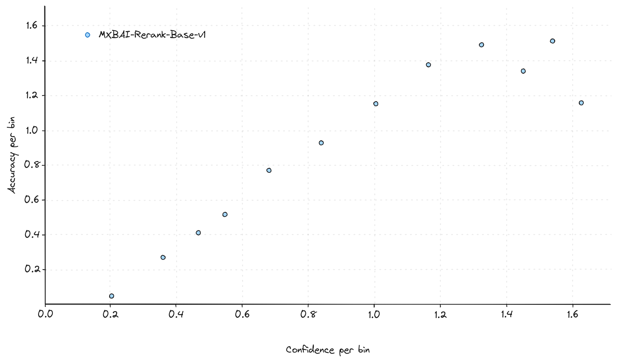
Figure 1 - Class Balanced Expected Calibration Error curve on MXBAI-Rerank-Base-v1 scores after min-max scaling on msmarco-v2
We'll discuss this further to explore how this can serve as a good calibration tool and what kind of sanity check we can use to evaluate the calibration potential of a given model.
How to calibrate your model
So far, we’ve introduced a metric, , which can be used to assess how well calibrated a model’s scores are on an understandable scale. In the following sections we’ll show how to use this to measure how well a model can be calibrated. First let’s clarify exactly what the understandable scale means.
For the simple case we have binary labels (0 meaning irrelevant, 1 meaning relevant), if we look at a group of query-document pairs that score around confidence 0.8, we would expect about 80% of those pairs to be relevant and 20% to be irrelevant. The metric checks how closely our expectations match reality. In other words, it measures the difference between what we expect and what we actually observe. For other labeling scales, it measures how well the expected scores match the labeling scale.
Even if your model isn’t perfectly calibrated, helps you connect your scores to real-world outcomes. It means that, eventually, you can scale your scoring system to reflect real accuracy levels. However, as we’ll see later, this isn’t always easy, especially if your model doesn’t have a smooth, increasing pattern in its predictions. But let’s assume we have a solid re-ranker model, like Elastic Rerank, and we want to set a threshold score where we expect the labels of re-ranked examples to be around 1.0 on msmarco-v2. Below, we’ll show a visual guide to what we’re trying to achieve.
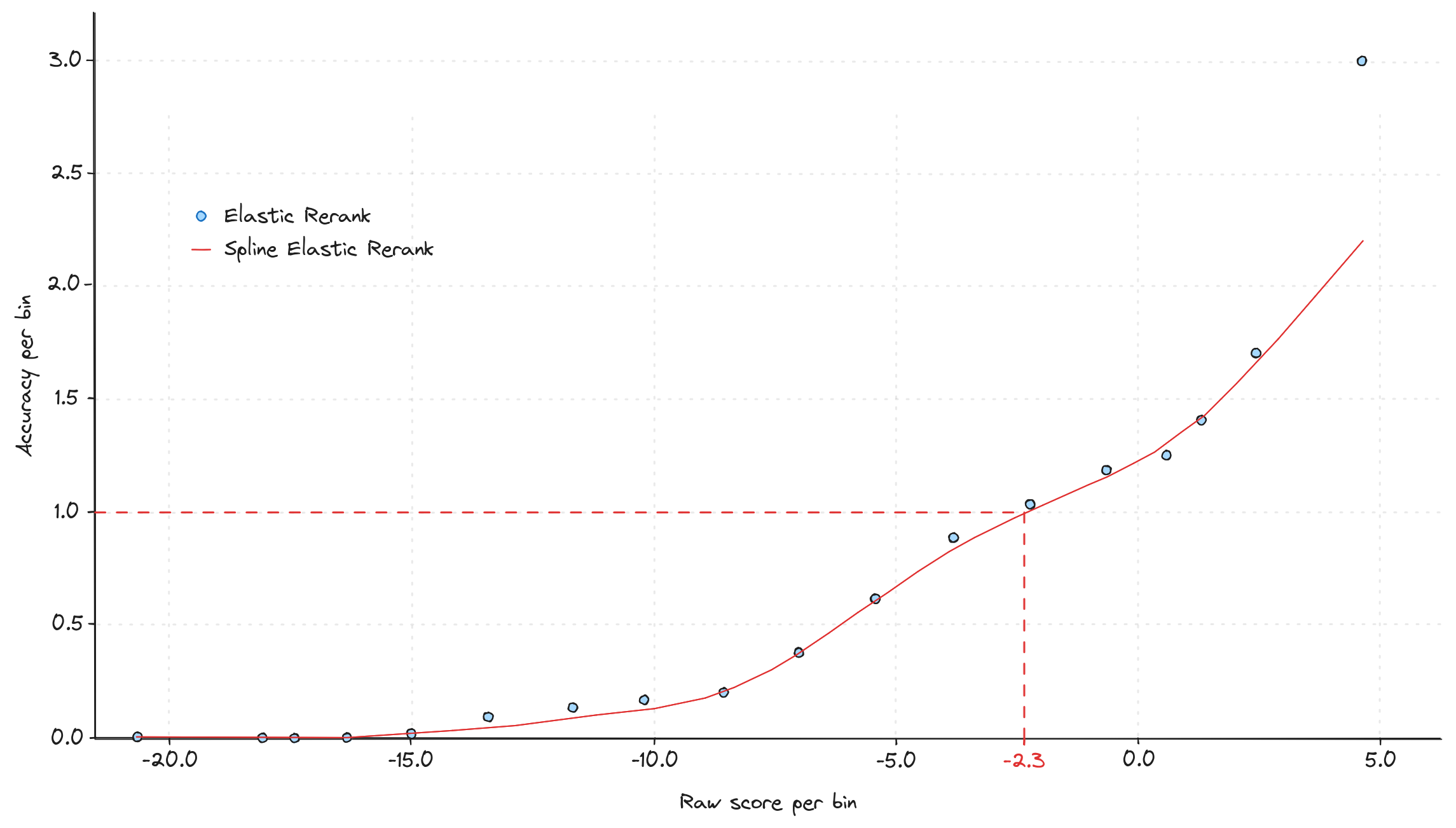
Figure 2 - Elastic Rerank calibration with cubic spline interpolation on msmarco-v2 (min-max scaling reverted)
Here, we use the curve, after reversing the min-max scaling, to predict the threshold that achieves our target. A cubic spline was chosen to reduce the risk of overfitting to noise. The smoothing parameter was determined through Bayesian optimization, minimizing the Mean Square Error between the spline interpolation computed on random small subsets (10% of the full dataset) and the actual accuracies measured on the remaining pairs, i.e. essentially by cross-validation. Notably, this smoothing parameter is relatively high, indicating that we can’t exactly fit the accuracies we measure on a subsample of the data because they wouldn’t generalize to new data. Please note that not all points carry the same weight, as this depends on labeling. The fit process accounts for these bin weights. Also, any negative accuracy value is clipped to 0, as negative accuracy is not meaningful.
This approach is especially useful because it doesn’t require a lot of annotations (as we will see below), works well even with unbalanced labeling, and is easy to adapt to different scoring scales (labels don’t have to be binary).
Sensitivity study and transferability
One of the assumptions we made earlier is that we have an annotated dataset. As always, this is a challenge, since doing it right is neither easy nor cheap. A key question to ask here is: “How many annotated query-document pairs do I need for this method to work?” While the answer will depend on factors like the level of annotation detail and the type of dataset, we conducted an ablation study using the msmarco-v2 dataset. It uses a 4-level annotation system (0: irrelevant, 1: related but not useful, 2: related but incomplete, 3: related and complete). The goal of the study was to look at the first and third quartile of measured cutoffs along the whole score range. We use the same strategy described above with a fixed smoothing parameter for cubic spline interpolation.
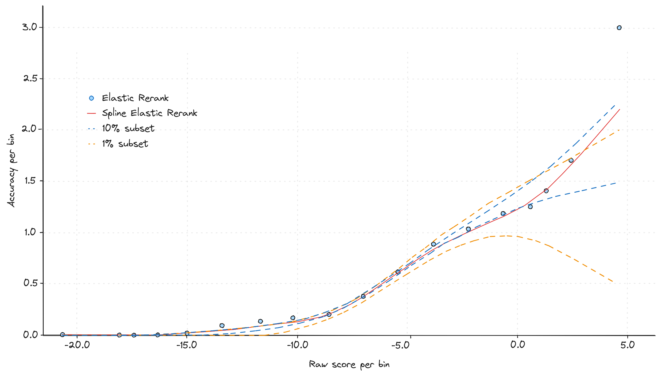
Figure 3 - Sensitivity study of the calibration of Elastic Rerank scores on msmarco-v2 as a function of the labeled data set size
An ablation rate of 90% means we're using 10% of the full msmarco-v2 dataset, while an ablation rate of 99% corresponds to using only 1% of the annotations. For each ablation rate, we conducted 20 random samples of the entire dataset. As shown, ablations do not impact estimations evenly across the score range. High cutoffs are particularly noisy at both ablation rates, likely due to a lower number of positive markups compared to negative ones, indicating that high score cutoffs may be unreliable without adequate annotations. At the 99% ablation rate, cutoffs lack precision, which could be because those 200 random annotations are not well enough chosen in our experiment, but it could also suggest that a few thousand annotations are probably the right order of magnitude to expect accurate estimations. That said, gathering 2,000 annotations is a realistic goal, especially if a large language model (LLM) is used to speed up the process.
Another question to consider is how transferable these thresholds are. For example, if you estimate a threshold using msmarco-v2, could that same threshold be applied to a different dataset (assuming you’ve reconciled label scales)? To explore this, we compared the Elastic Rerank curve on msmarco-v2 and on robust04, another dataset from the BEiR collection, to see how well the thresholds hold up across datasets. Note that we scaled accuracy to 0-1 to simplify comparison of both datasets.
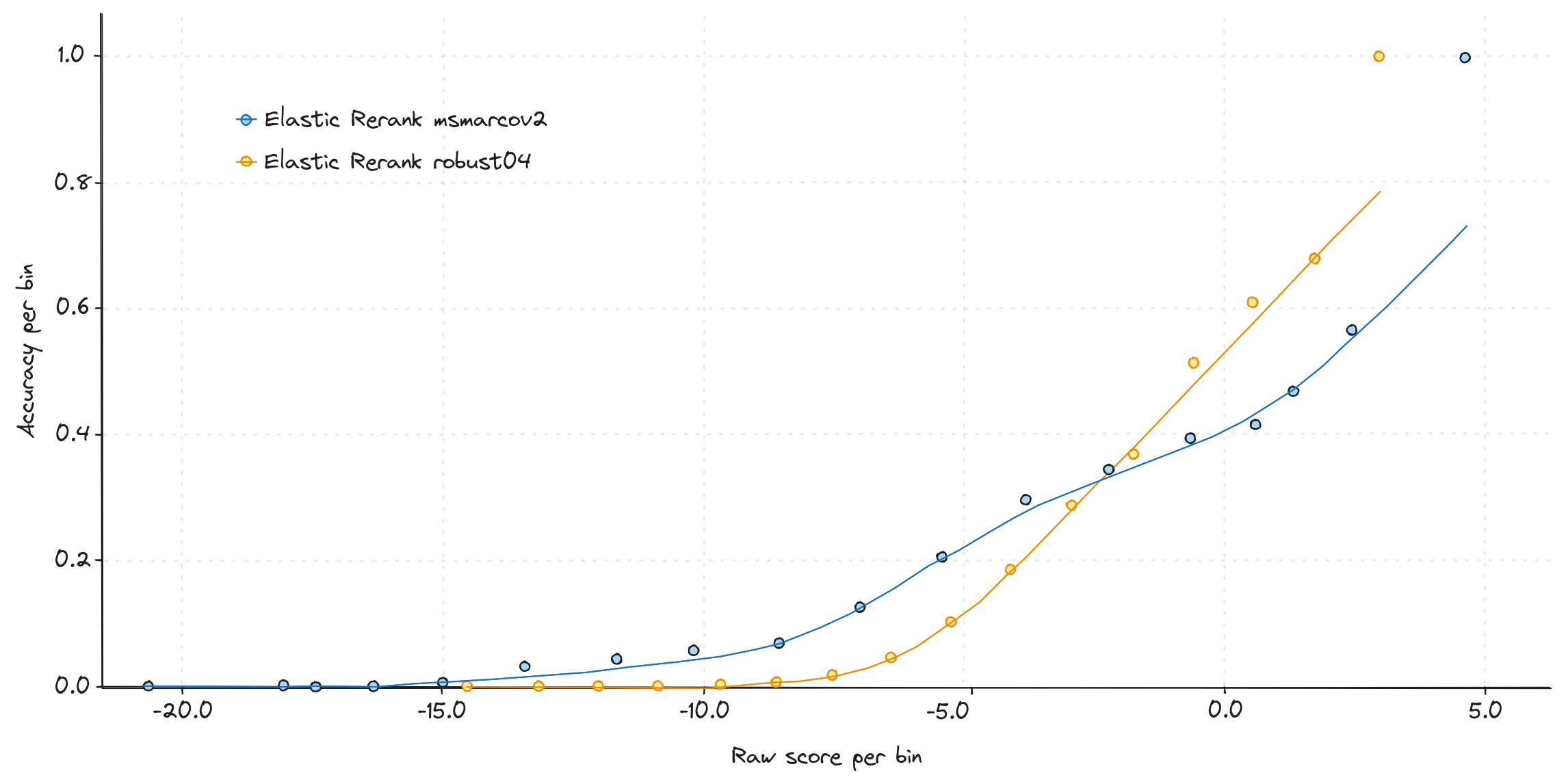
Figure 4 - Elastic Rerank calibration with cubic spline interpolation on robust04 and msmarco-v2
Unfortunately, as we can see in Figure 4, although the curves are qualitatively similar, we can’t reliably apply a threshold calculated from one dataset to another. This difficulty may stem from differences between datasets or variations in evaluators (or their guidelines) used to generate the label data. Even minor shifts in the interpretation of scale can lead to significant differences in thresholds. Ultimately, both factors suggest that using a more “stable” annotator—such as an LLM with a consistent prompt (with a human in the loop to double-check annotations)—on your specific dataset would allow for much more precise calibration.
Sanity check and conclusion
In the end, as we discussed earlier, the effectiveness of this method heavily relies on the quality of your model. A poorly performing model will show inconsistent behavior between different query samples, making it difficult to reliably predict a threshold for any given scale. We want to assess that by evaluating how predictions will work on unseen data. One way to achieve this is by using a modified version of . Rather than assessing the error between observed confidence and accuracy within each bin, we can evaluate the error between predicted confidence and accuracy per bin. Put simply, this metric captures the difference between observed confidence and the spline model’s predictions (see Figure 5). Note that the spline model is effectively a cross-validated confidence predictor from the raw model scores.
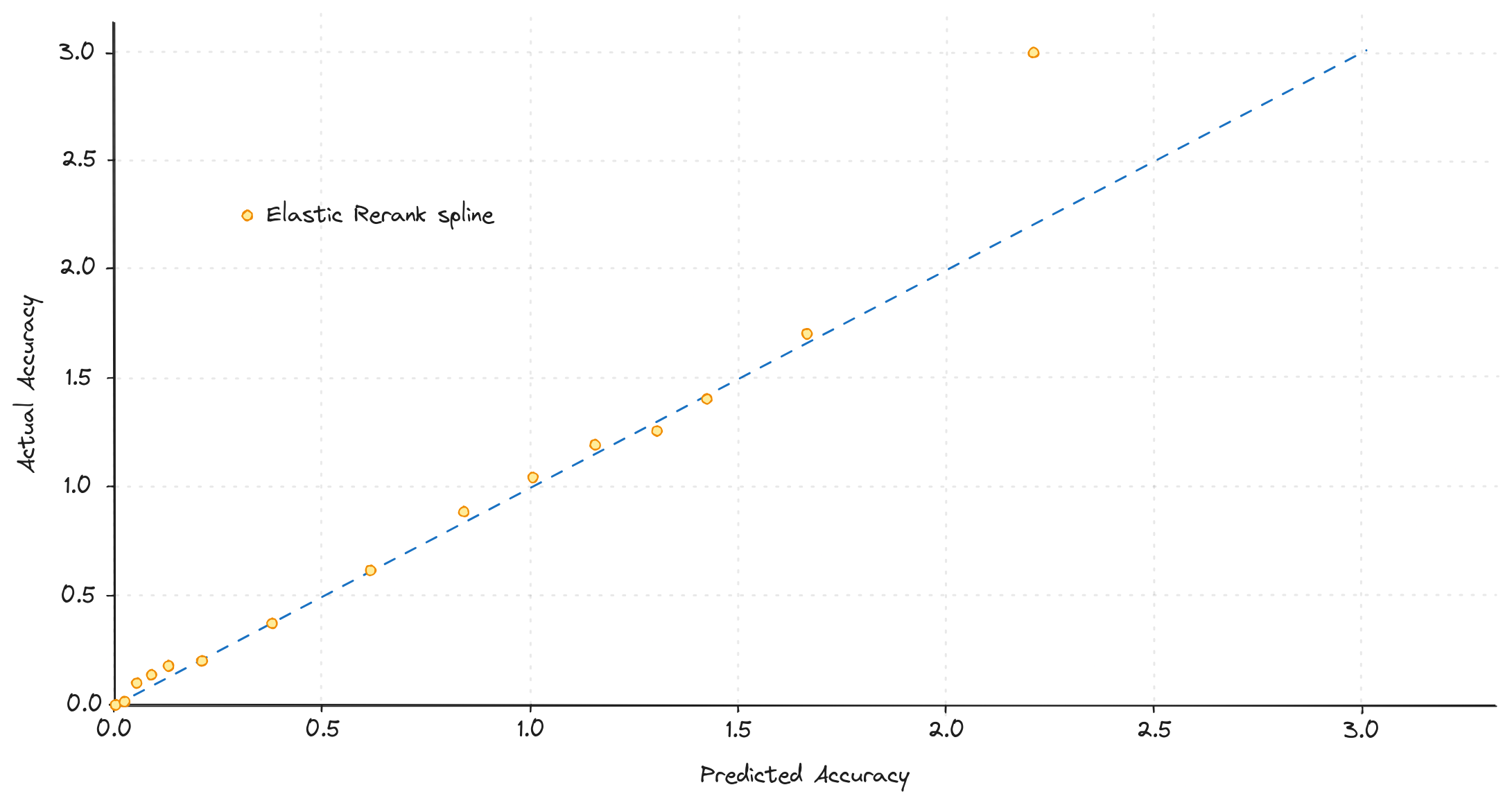
Figure 5 - Elastic Rerank sanity check between spline predictions and measured points
This approach makes it straightforward to quickly assess if our calibration model will perform as expected. We measured this modified for three models: Elastic Rerank, MXBAI-rerank-v1, and BGE-gemma-v2. Ideally, calibration quality should correlate with each model's ranking quality. From prior analysis, we know that MXBAI-rerank-v1 is a weaker re-ranker compared to BGE-gemma and Elastic Rerank (which we expect to perform similarly). This is precisely what we observed on the msmarco-v2 dataset (see Figure 6).
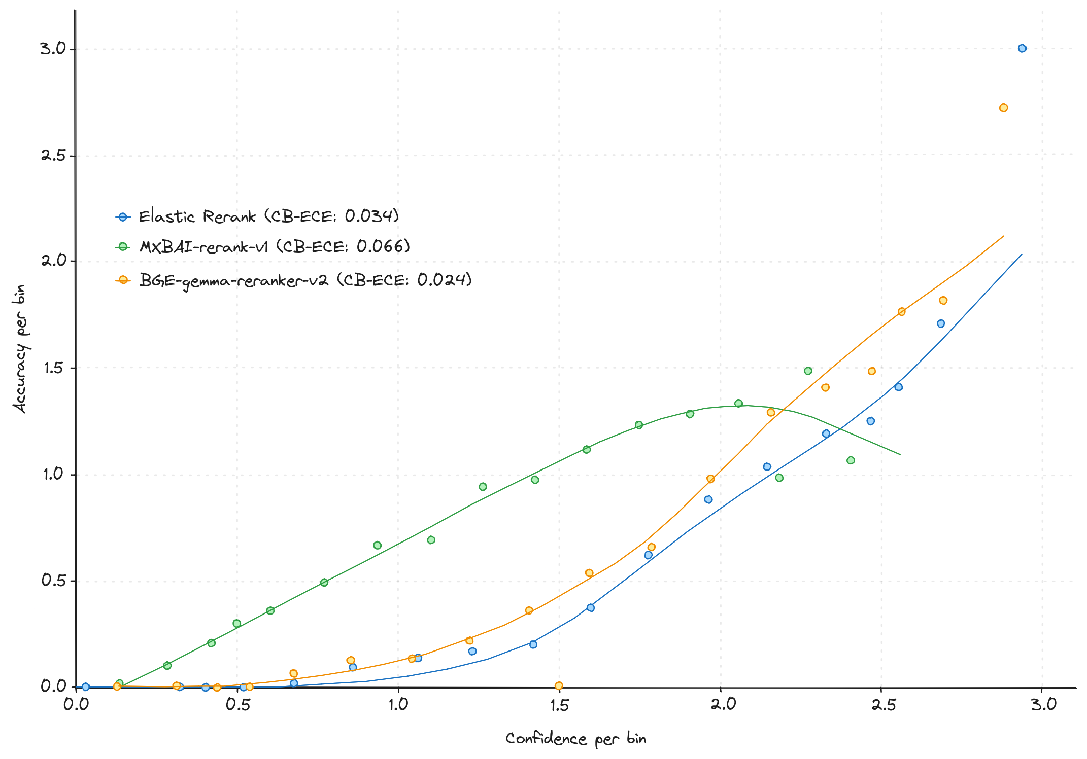
Figure 6 - Elastic Rerank, Gemma and MXBAI re-rankers comparison (lower CB-ECE is better)
In conclusion, we’ve explored a method for defining clear cut-offs based on real-world requirements that can be mapped to model scores. We roughly estimated the annotation volume needed, a few thousand labels to achieve high accuracy, and introduced metrics to gauge the reliability of these estimates. This type of analysis could be seen as a way to evaluate models from a different perspective, beyond traditional ranking metrics like NDCG.
Ready to try this out on your own? Start a free trial.
Want to get Elastic certified? Find out when the next Elasticsearch Engineer training is running!
Related content

September 15, 2025
Balancing the scales: Making reciprocal rank fusion (RRF) smarter with weights
Exploring weighted reciprocal rank fusion (RRF) in Elasticsearch and how it works through practical examples.

September 8, 2025
MCP for intelligent search
Building an intelligent search system by integrating Elastic's intelligent query layer with MCP to enhance the generative efficacy of LLMs.

Building intelligent duplicate detection with Elasticsearch and AI
Explore how organizations can leverage Elasticsearch to detect and handle duplicates in loan or insurance applications.
July 10, 2025
Diversifying search results with Maximum Marginal Relevance
Implementing the Maximum Marginal Relevance (MMR) algorithm with Elasticsearch and Python. This blog includes code examples for vector search reranking.

July 9, 2025
Semantic text is all that and a bag of (BBQ) chips! With configurable chunking settings and index options
Semantic text search is now customizable, with support for customizable chunking settings and index options to customize vector quantization, making semantic_text more powerful for expert use cases.