Introduction
In this blog post, I'll demonstrate the process of loading, analyzing, and visualizing data using Elasticsearch, Python, and Kibana. While the examples will revolve around Boston Celtics data, the techniques and concepts can be applied to other datasets. You can view the complete code for this blog post.
The choice to use Boston Celtics' data stemmed from a personal experience. I was going through a stressful time about a year ago and ended up at a basketball game. For the entire time, I could disconnect and find focus in a way I hadn't previously been able to. The first team that I got into was the Boston Celtics. The Boston Celtics are an unusual team, and while they've often been at the top of power rankings for the NBA this season, they only sometimes lead the league in many core metrics.
Using data visualization, I could dive deeper into this team, answer some critical questions about it, and analyze the season better.
Steps to analyze data using Python, Elasticsearch & Kibana
Prerequisites
- This tutorial uses Elasticsearch version 8.11; if you are new, check out our Quick Starts on Elasticsearch and Kibana.
- Download the latest version of Python if you don’t have it installed on your machine. This example utilizes Python 3.12.1.
- You will use the nba_api package to get recent statistics about the Boston Celtics, Jupyter Notebooks, and the Elasticsearch Python Client. While testing this code, I got an error unless I had pandas installed since the nba_data creates pandas DataFrames.
To install these packages, you can run the following command.
pip3 install nba_api jupyter elasticsearch pandas- You will want to load a Jupyter Notebook to work with your data interactively. To do so, you can run the following in your terminal.
jupyter notebookIn the right-hand corner, you can select where it says “New” to create a new Jupyter Notebook.
Step 1: Parsing and cleaning the data
The first step will be to connect to NBA data and load that data into Elasticsearch. You will first need to import the required libraries. For this example, you will use nba_api’s static team data to get information about the Boston Celtics. The leaguegamefinder endpoint allows you to get information. To connect to Elastic, you will use the Elasticsearch Python Client, elasticsearch. To enter your passwords via an interactive prompt, you’ll use getpass.
To load these packages, you can use the following code:
from nba_api.stats.static import teams
from nba_api.stats.endpoints import leaguegamefinder
from elasticsearch import Elasticsearch, helpers
from getpass import getpass
You will want to get the team data from the NBA team static dataset, which has an ID for each team. You can use a list comprehension to find the team with the abbreviation of BOS for Boston. Once you get the complete Celtics object, you can narrow it down to just the ID, which you can use to find game data.
nba_teams = teams.get_teams()
celtics = [team for team in nba_teams if team['abbreviation'] == 'BOS'][0]
celtics_id = celtics['id']
Now, you can use the Celtics' ID to get all the available game data for the team. You view the first five results to ensure the data was correctly loaded using the .head() method.
celtics_games = leaguegamefinder.LeagueGameFinder(team_id_nullable=celtics_id)
games = celtics_games.get_data_frames()[0]
games.head()
While working with this data, I noticed that data for the year includes pre-season data. So, I used the season dates to narrow the data down to the current season. In a Jupyter Notebook, you can call current_season to view the full DataFrame.
current_season = games.loc[(games['GAME_DATE'] >= '2023-10-24') & (games['GAME_DATE'] <= '2024-06-20')]
current_season
Since null values can create issues when loading your data to Elasticsearch, you can double-check that this data has none. The line below returns a boolean value, letting you know if your data has any null values. Since this dataset returns a value of False, it has no null values, so we don't have to do further cleaning.
current_season.isnull().values.any()Step 2: Loading the data into Elasticsearch
After parsing the NBA data and finishing cleaning your data, you can create variables for your Elastic Cloud ID and Elastic API Key. Using getpass, you can securely enter your credentials.
elastic_cloud_id = getpass("Elastic Cloud ID: ")
elastic_api_key = getpass("API Key: ")
Once you've entered your credentials, you can connect to Elasticsearch using the elasticsearch client.
es = Elasticsearch(cloud_id=elastic_cloud_id, api_key=elastic_api_key)Before you can load your data into Elastic, you must create an index. You can create one for the current season.
es.indices.create(index="boston_celtics_current_season")You can create a function to load data from the current season into Elasticsearch. Each game is considered a document.
timeframe = 'boston_celtics_current_season'

def doc_generator(df, timeframe):
    for index, document in df.iterrows():
        yield {
            "_index": timeframe,
            "_id": f"{document['GAME_ID']}",
            "_source": document.to_dict(),
        }
The helpers feature of the Python client allows you to efficiently upload your DataFrame, which holds data on the current season's games, into Elasticsearch. By calling the doc_generator function you just created, you can convert your DataFrame into documents.
helpers.bulk(es, doc_generator(current_season, timeframe))Step 3: Writing queries with Elasticsearch
Now that your data is loaded, you can start writing queries with Elasticsearch to learn more about how the Boston Celtics perform this season. First, you can create a query to see how many wins they have had so far this season and return the count of wins as a result.
search_query = {
    "query": {
        "match": {
            "WL": "W"
        }
    }
}

games_won = es.count(index="boston_celtics_current_season", body=search_query)
While working with complex datasets, writing sentences to help explain the dataset is sometimes helpful. Here is one example of how many games the Boston Celtics have won this season.
print(f"The Celtics won {games_won['count']} games this season so far.")The output should look something like this:
The Celtics won 29 games this season so far.A streak in sports refers to a consecutive series of games or events in which a team or individual consistently wins or loses. Streaks are significant because they reflect a period of either exceptional performance (winning streak) or a challenging phase (losing streak). While analyzing how well a team is performing, examining how many streaks they have is often helpful. You can create a query that allows you to sort the wins and losses by game data.
streak_query = {
  "size": 1000,
  "sort": [
    {
      "GAME_DATE": {
        "order": "asc"
      }
    }
  ],
  "_source": ["GAME_DATE", "WL"]
}
You can use the es.search() method to create a search based on the query above.
streak_search = es.search(
    index="boston_celtics_current_season",
    body=streak_query)
The following code creates a JSON object of game date with the game result.
gs = [hit['_source'] for hit in streak_search['hits']['hits']]To view the top five streaks of the season, you can create a dictionary of each streak and sort it accordingly.
streaks = []
current_streak = 1
for i in range(1, len(gs)):
    if gs[i]['WL'] == gs[i-1]['WL']:
        current_streak += 1
    else:
        streaks.append((gs[i-1]['WL'], current_streak))
        current_streak = 1


streaks.append((gs[-1]['WL'], current_streak))
top_streaks = sorted(streaks, key=lambda x: x[1], reverse=True)[:5]
top_streaks
Step 4: Creating a dashboard with Kibana
While we can continue writing queries to learn more about the Boston Celtics, creating a dashboard is a more efficient way to draw insights from your data.
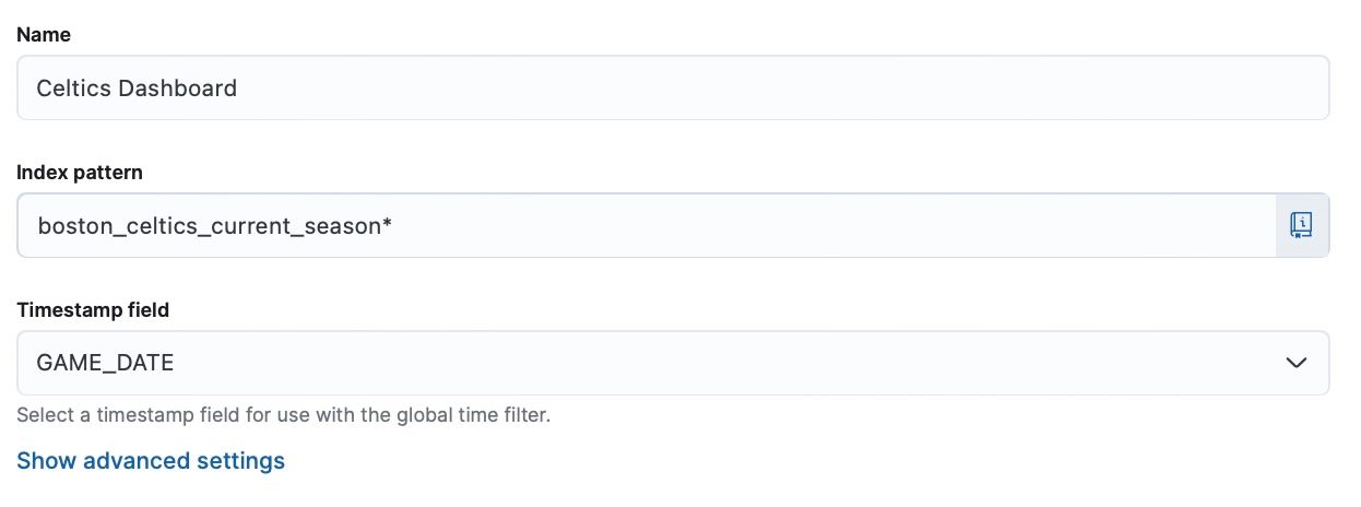
Before making a dashboard, you will need to create a data view to ensure Kibana can access the data in your Elasticsearch index. For your data view, you will need to give it a name, select the index or pattern representing multiple indices you want to visualize and provide a timestamp field so you can create time-based visualizations.
After you've created a data view, you can start to create a dashboard. Under the header "Analytics," select where it says "Dashboard," and click where it says "Create Dashboard."
An excellent visualization to start with is creating a title visualization for your dashboard. You can select a text visualization and markdown to add an image to the title.
#  How are the Boston Celtics performing this season?
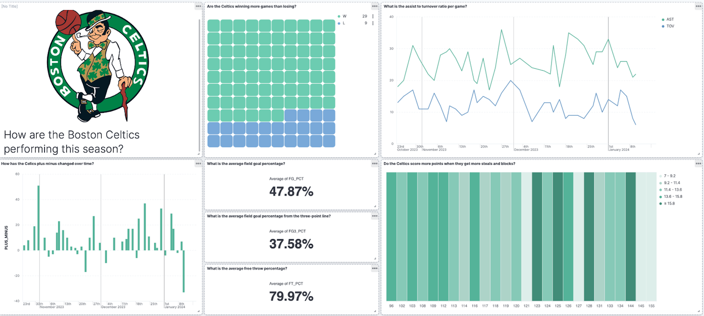
To learn if the Celtics are winning more games than losing, you can create a waffle chart to illustrate that at this point in the season, the Celtics are winning more games than losing.
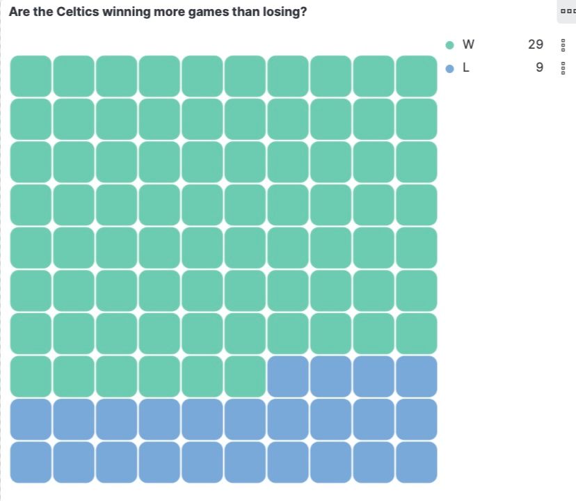
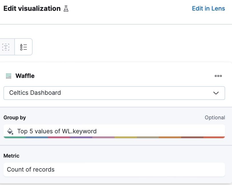
You can see the configuration of this chart here:
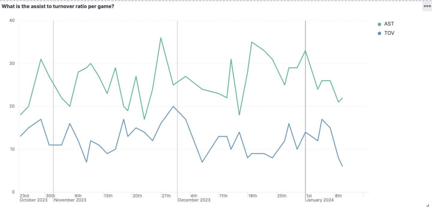
Maintaining more assists than turnovers is a crucial indicator of effective ball movement within a team. The accompanying visualization, current as of the date of this blog post, clearly illustrates that the team is performing well in this aspect, showcasing proficient ball distribution and teamwork.
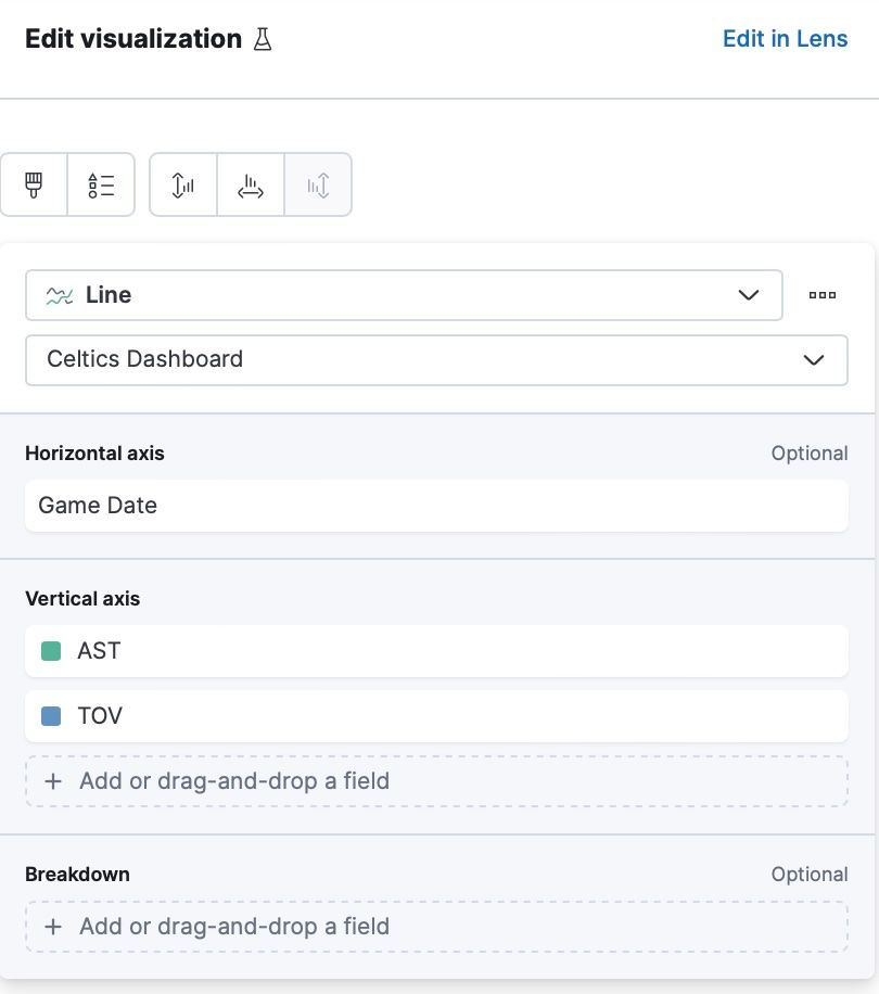
The configuration of this visualization looks like this:
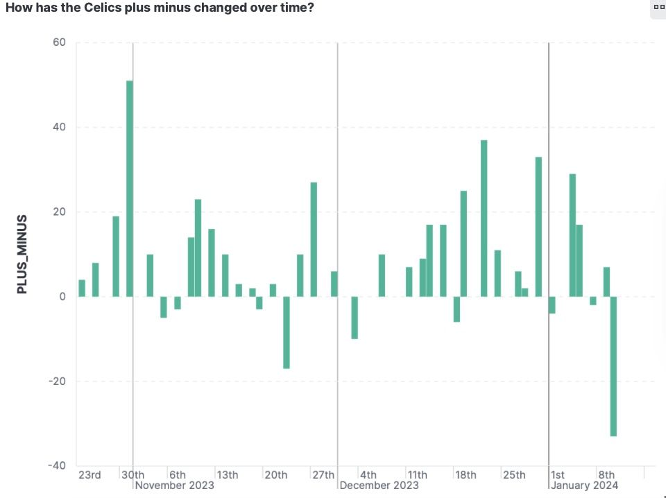
The plus-minus in basketball shows how many more points the Boston Celtics had over the other team, this statistic is often used to explain the impact a team has had on the game. A high plus score indicates that the team tends to do well in terms of scoring or preventing goals/points when that team is playing. A high minus score suggests the opposite – that the team tends to be outscored. At the beginning of season there was an outlier with one game where the Celtics scored over 50 points more than the other team but this normalized over time. The most recent game (at the time of writing), against the Milwaukee Bucks was also an outlier as well.
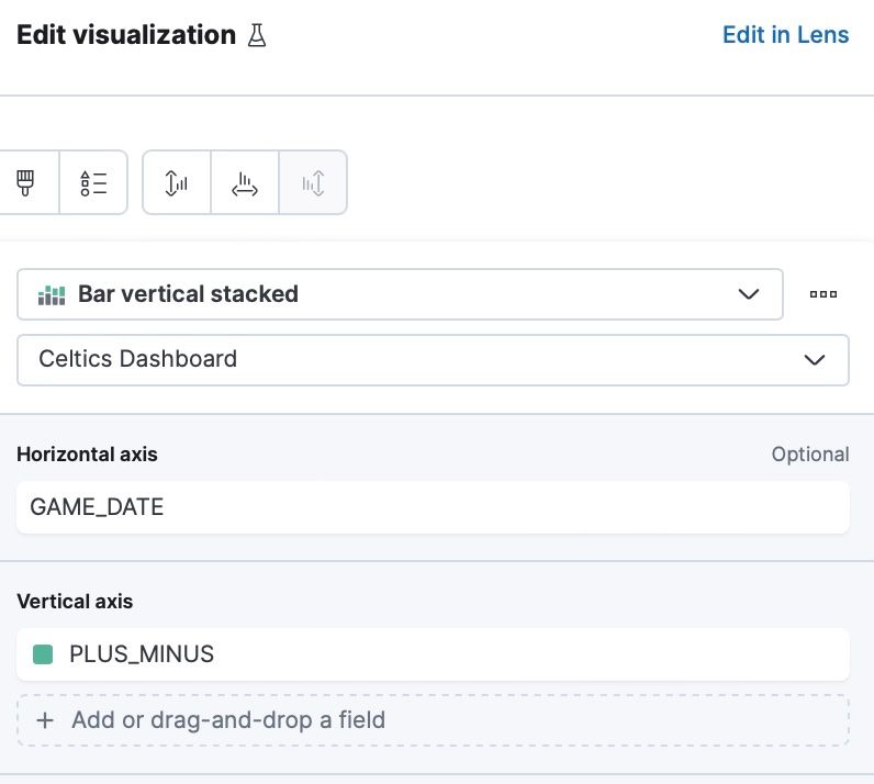
Below is the configuration of the above visualization.
To learn more about how often the Celtics are making shots, you can create a few top lines, including:
- What is the average field goal percentage?
- What is the average field goal percentage from the three-point line?
- What is the average free throw percentage?
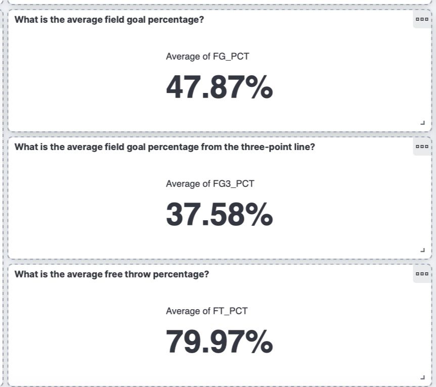
The configuration of these top lines looks like this in Kibana:
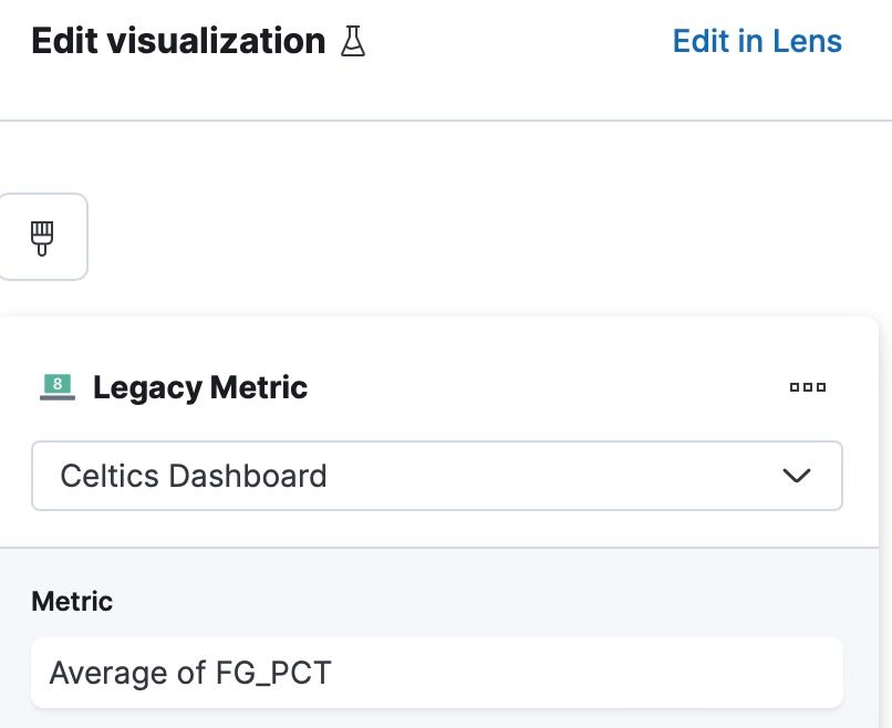
Configuration of field goal percentage topline:
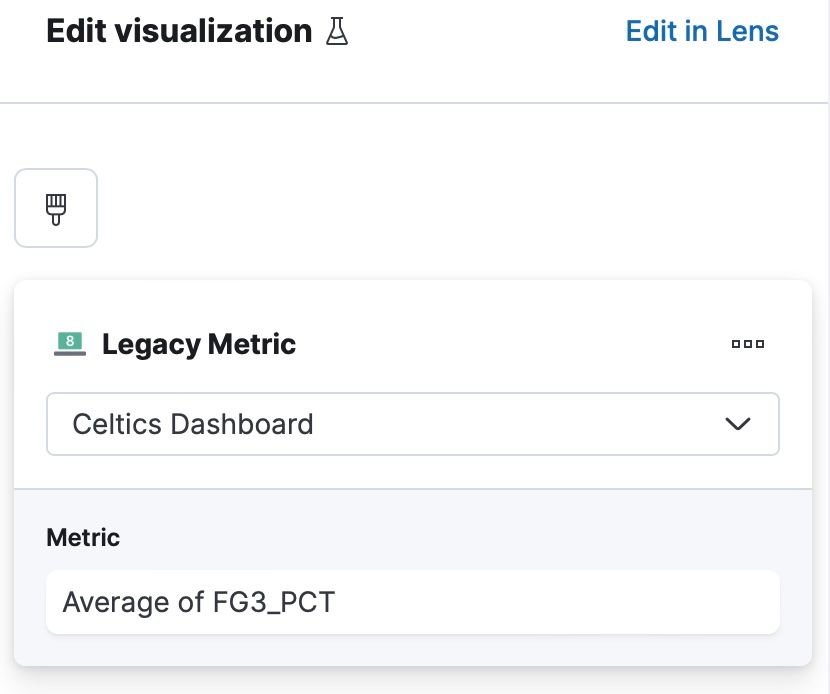
Configuration of field goal percentage from the three point line topline:
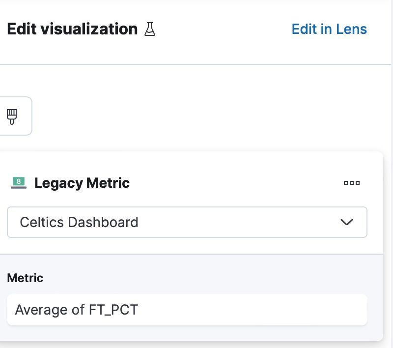
Configuration of free throw percentage topline:
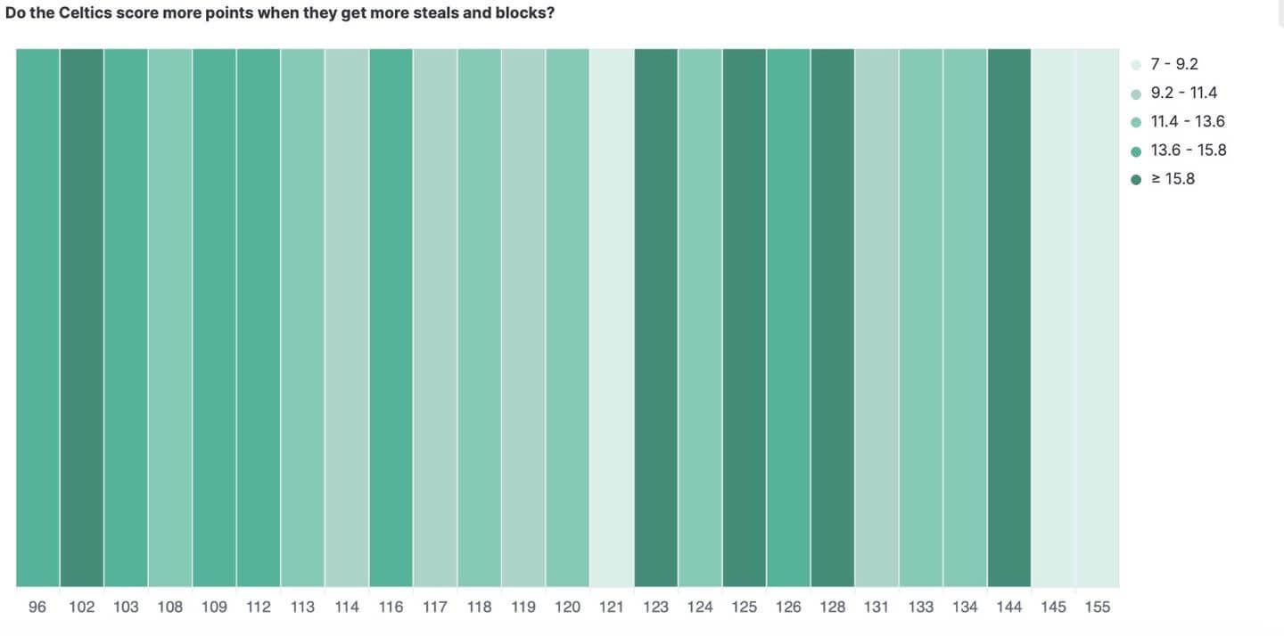
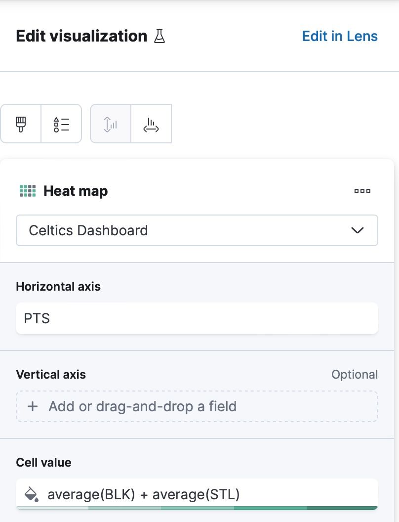
The final visualization examines whether the Celtics' scoring increases with more steals and blocks. The colors represent the average of blocks plus the average of steals. The green gets dark as the number of blocks and steals increases. However, the absence of a discernible pattern in the data suggests no significant correlation between these defensive actions and their overall scoring.
The configuration of this visualization should look like this:
Conclusion
By visualizing data in this way, you can robustly interact with your data and draw further insights. Be sure to check out the complete code for this blog post. As a next step, create a data pipeline to programmatically get the data into your dashboard or utilize some of our machine learning features, such as anomaly detection. You also can expand this dataset by adding historical Celtics data or comparing the Celtics to other teams across the NBA. We hope you can continue to use Python, Elasticsearch, and Kibana. As always, let us know if you need if this blog post inspires you to build anything or if you have any questions on our Discuss forums and the community Slack channel.
Ready to try this out on your own? Start a free trial.
Want to get Elastic certified? Find out when the next Elasticsearch Engineer training is running!
Related content

October 15, 2025
Training LTR models in Elasticsearch with judgement lists based on user behavior data
Learn how to use UBI data to create judgment lists to automate the training of your Learning to Rank (LTR) models in Elasticsearch.

September 19, 2025
Using TwelveLabs’ Marengo video embedding model with Amazon Bedrock and Elasticsearch
Creating a small app to search video embeddings from TwelveLabs' Marengo model.

Using LangExtract and Elasticsearch
Learn how to extract structured data from free-form text using LangExtract and store it as fields in Elasticsearch.

Introducing the ES|QL query builder for the Python Elasticsearch Client
Learn how to use the ES|QL query builder, a new Python Elasticsearch client feature that makes it easier to construct ES|QL queries using a familiar Python syntax.
Evaluating your Elasticsearch LLM applications with Ragas
Assessing the quality of a RAG solution using Ragas metrics and Elasticsearch.