Recently, we introduced optimized scalar quantization (OSQ) and donated it to Lucene. This powers our implementation of binary quantization (BBQ). As we continue on our journey to make BBQ the default format for all our vector indices, we’ve been exploring its robustness across a wider range of data characteristics.
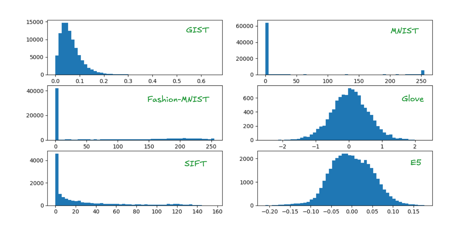
As we discussed before, many high quality learned embeddings share a similar characteristic: their components are normally distributed. However, classic approximate nearest neighbor (ANN) benchmark datasets often do not share this characteristic.
In this blog, we explore:
- The distribution characteristics of a variety of classic ANN benchmark datasets,
- How they perform with vanilla OSQ, and
- The effect of a preconditioner on retrieval robustness.
We propose a sparse variant of the random orthogonal preconditioner introduced by RaBitQ, which achieves similar quality, but at a fraction of the cost.
Datasets
In this study we use a subset of the datasets included in the popular ann-benchmark suite:
- GIST that contains 960 handcrafted features for image recognition
- MNIST and Fashion-MNIST that are 2828 images whose grayscale pixel values comprise the 784 dimensional vectors
- GloVe that comprises a collection of unsupervised word vector embeddings, and
- SIFT that contains 128 handcrafted image descriptors
We also include some embedding model based datasets to understand the impact we have on these if any:
- e5-small embeddings of the quora duplicate question dataset
- Cohere v2 embedding of a portion of the wikipedia dataset
These have diverse characteristics. Some of their high-level features are summarized in the following table.
| Dataset | Dimension | Document count | Metric |
|---|---|---|---|
| GIST | 960 | 1000000 | Euclidean |
| MNIST | 784 | 60000 | Euclidean |
| Fashion-MNIST | 784 | 60000 | Euclidean |
| Glove | 100 | 1183514 | Cosine |
| SIFT | 128 | 1000000 | Euclidean |
| e5-small | 384 | 522931 | Cosine |
| Cohere v2 | 768 | 934024 | MIP |
The figures below show sample component distributions.
Preconditioning
RaBitQ proposes random orthogonal preconditioning as an initial step for constructing quantized vectors. An orthogonal transformation of a vector corresponds to a change of basis. It is convenient in the context of quantization schemes because it doesn’t change the similarity metric. For example, for any orthogonal matrix P the dot product is unchanged since
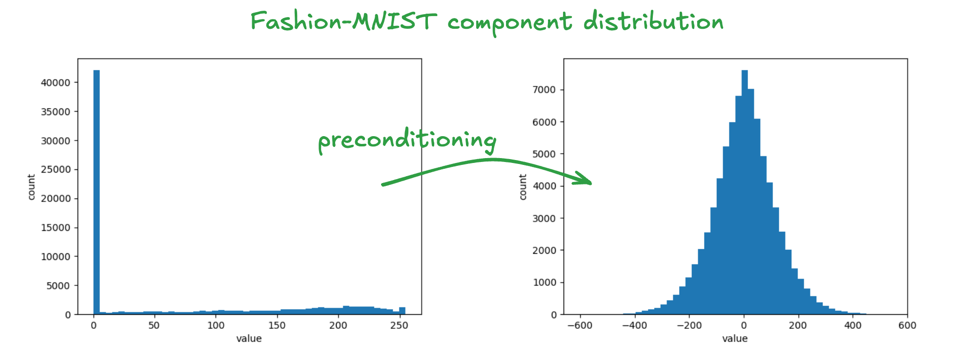
The same holds for cosine similarity and Euclidean distance. So the transform can just be applied to each vector before quantizing it and no further changes are needed to either the index or query procedure. For our purposes, another important property of this transformation is that it makes the component distributions more normally distributed. This is a consequence of the central limit theorem. Specifically, the component of the transformed vector corresponds to the summation where are approximately independent random variables. It is easy to sample such a matrix: first sample elements independently from the standard normal distribution and then apply modified Gram-Schmidt orthogonalization to the resulting matrix (which is almost surely rank full). The figure below shows the impact of this transform on the component distribution when it’s applied to the Fashion-MNIST dataset.
This property suits OSQ because our initialization procedure assumes that the components are normally distributed. The resulting transformation is effective, but it comes with some overheads:
- The preconditioning matrix contains floating point values
- Applying the transformation to the full dataset requires floating point multiplications.
For example, if the vectors have 1024 dimensions, we’d require 4MB storage per preconditioning matrix and perform more than 1M multiplications per document we add to the index.
We therefore asked, “do we really need a dense orthogonal matrix to achieve our goal?” For high dimensional vectors we might reasonably expect that we can mix fewer components and still the resulting component distributions will be fairly normal. One way to achieve this is using a block diagonal matrix as illustrated schematically below.
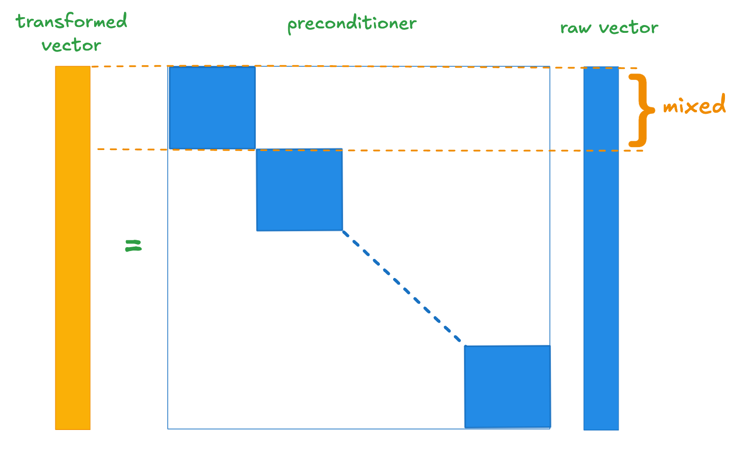
If we use a block diagonal matrix whose blocks are we drop the memory requirement for a dimensional preconditioner to and we reduce the indexing overhead by a factor of 32. This is pretty appealing.
Although the vanilla block diagonal preconditioner performs fairly well, it gives up some of the recall gains we achieve with a dense preconditioner. Furthermore, the choice of a block diagonal matrix is arbitrary: it is mixing components that happen to be adjacent to each other in the vector. It seems undesirable that the effectiveness of our scheme might change for an arbitrary permutation of the input vectors. Ideally we would use a procedure which yields a deterministic choice for which components we mix.
To do this we drew inspiration from optimized product quantisation. This seeks to balance variance between groups of components used to build each codebook. In a similar vein, we use a greedy algorithm to assign components to blocks with the aim to balance their variance as follows.
for
while in descending component variance order
Add to
if
Add the variance of the component to
else
Here, is the vector dimension and is the block dimension. Our intuition is that this should maximize the homogeneity of component distributions and that this is beneficial because we use the same quantization interval for each component. This intuition is borne out by the results. We achieve similar quality to the dense transformation at a fraction of the cost.
Results
As is typical, we evaluate recall reranking some collection of vectors larger than the number of required candidates. The following table breaks down the recall@10 at 5 distinct reranking depths for the most challenging vector distributions in our test set with and without preconditioning. It also compares dense preconditioning with the optimized block diagonal preconditioning we described above, using a block size of 32. Averaged across datasets and reranking depths we see an increase in recall of 31% using block diagonal preconditioning for these datasets compared to the baseline. It’s also clear that the block diagonal preconditioner with balanced variance is on a par with the dense preconditioner.
| Dataset | Metric | Baseline | Dense preconditioner | Sparse preconditioner |
|---|---|---|---|---|
| Fashion-MNIST | recall@10|10 | 0.444 | 0.712 | 0.710 |
| recall@10|20 | 0.629 | 0.911 | 0.911 | |
| recall@10|30 | 0.730 | 0.964 | 0.966 | |
| recall@10|40 | 0.792 | 0.983 | 0.984 | |
| recall@10|50 | 0.833 | 0.990 | 0.992 | |
| MNIST | recall@10|10 | 0.544 | 0.795 | 0.787 |
| recall@10|20 | 0.719 | 0.970 | 0.967 | |
| recall@10|30 | 0.800 | 0.994 | 0.993 | |
| recall@10|40 | 0.848 | 0.998 | 0.998 | |
| recall@10|50 | 0.880 | 0.999 | 0.999 | |
| GIST | recall@10|10 | 0.314 | 0.558 | 0.545 |
| recall@10|20 | 0.438 | 0.746 | 0.739 | |
| recall@10|30 | 0.521 | 0.837 | 0.825 | |
| recall@10|40 | 0.581 | 0.884 | 0.878 | |
| recall@10|50 | 0.625 | 0.916 | 0.911 | |
| SIFT | recall@10|10 | 0.243 | 0.272 | 0.264 |
| recall@10|20 | 0.351 | 0.395 | 0.382 | |
| recall@10|30 | 0.425 | 0.477 | 0.461 | |
| recall@10|40 | 0.478 | 0.537 | 0.519 | |
| recall@10|50 | 0.522 | 0.584 | 0.565 |
Recall @10 for various reranking depths using raw OSQ and preconditioned OSQ (higher is better)
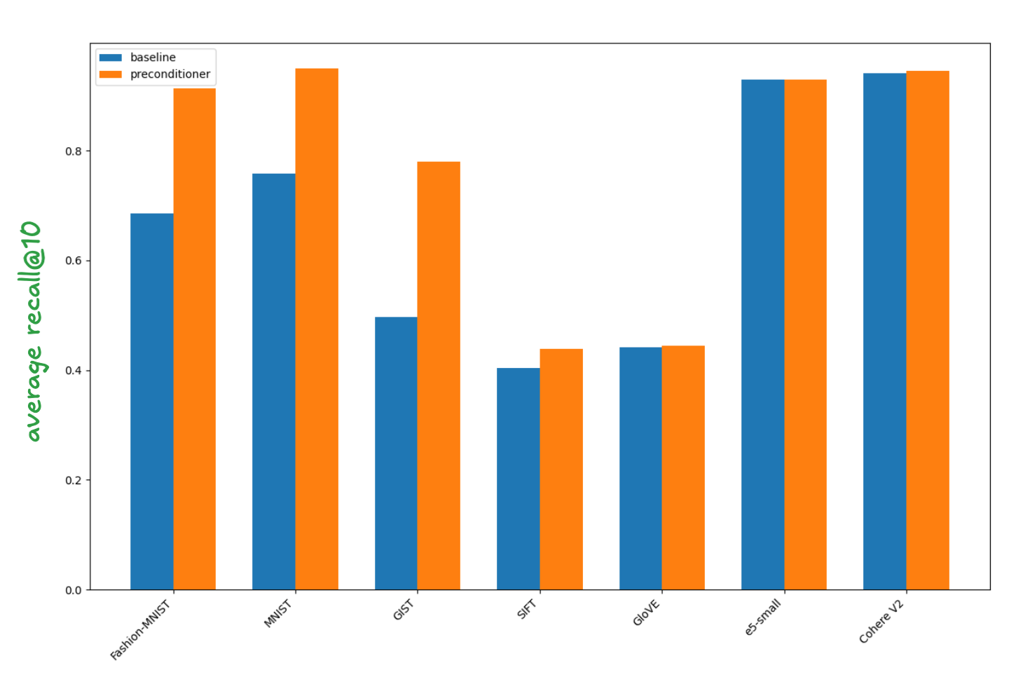
For completeness we show the average recall@10 across the five reranking depths for the baseline and block diagonal preconditioning across all the test datasets in the figure below. This shows that preconditioning is essentially a no-op on well behaved datasets.
In summary, the block diagonal preconditioner increases robustness with modest overhead.
Conclusion
Our SIMD accelerated binary quantization scheme has enabled us to achieve fantastic index efficiency and query recall-latency tradeoff. Our goal is to make this work easily consumable by everyone.
In this post we discussed a lightweight preconditioner we’re planning to introduce to the backing quantization scheme as we move towards enabling BBQ as the default format for all vector indices. This improves its robustness against pathological vector distributions for a small index time overhead.
Ready to try this out on your own? Start a free trial.
Elasticsearch has integrations for tools from LangChain, Cohere and more. Join our advanced semantic search webinar to build your next GenAI app!
Related content

December 19, 2024
Understanding optimized scalar quantization
In this post, we explain a new form of scalar quantization we've developed at Elastic that achieves state-of-the-art accuracy for binary quantization.
November 18, 2024
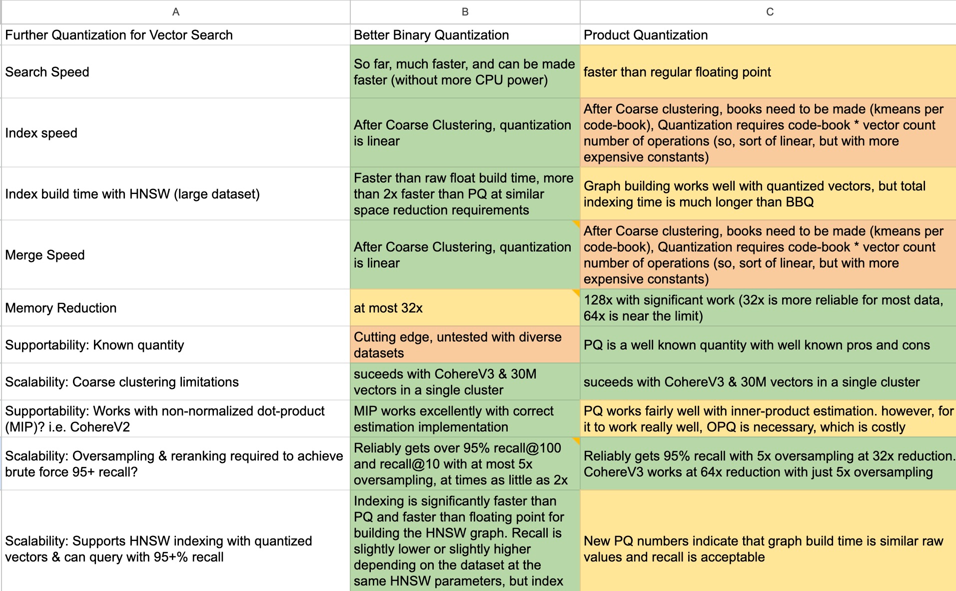
Better Binary Quantization (BBQ) vs. Product Quantization
Why we chose to spend time working on Better Binary Quantization (BBQ) instead of product quantization in Lucene and Elasticsearch.
December 4, 2024
Smokin' fast BBQ with hardware accelerated SIMD instructions
How we optimized vector comparisons in BBQ with hardware accelerated SIMD (Single Instruction Multiple Data) instructions.

April 15, 2025
Elasticsearch BBQ vs. OpenSearch FAISS: Vector search performance comparison
A performance comparison between Elasticsearch BBQ and OpenSearch FAISS.

May 3, 2024
Evaluating scalar quantization in Elasticsearch
Learn how scalar quantization can be used to reduce the memory footprint of vector embeddings in Elasticsearch through an experiment.