In Elasticsearch, a significant terms aggregation goes beyond the most common terms to find statistically unusual values in a dataset. This allows us to discover valuable insights and non-obvious patterns. A significant terms aggregation provides a response with two useful parameters:
- bg_count (background count): Number of documents found in the parent dataset
- doc_count: Number of documents found in the result dataset
For example, in a phone sales dataset, we can look for significant terms on the iPhone 16 sales like this:
GET phone_sales_analysis/_search
{
 "size": 0,
 "query": {
   "term": {
     "phone_model": {
       "value": "iPhone 16"
     }
   }
 },
 "aggs": {
   "significant_cities": {
     "significant_terms": {
       "field": "city_region",
       "size": 1
     }
   }
 }
}
Then, the response gives us:
{
 "aggregations": {
   "significant_cities": {
     "doc_count": 122,
     "bg_count": 424,
     "buckets": [
       {
         "key": "Houston",
         "doc_count": 12,
         "score": 0.1946481360617346,
         "bg_count": 14
       }

     ]
   }
 }
}
Houston is not in the top 10 of cities in the whole dataset nor the top city for the iPhone 16. However, the significant terms aggregation showed that the iPhone 16 is being bought disproportionately in this city compared to the rest of the data. Let’s dive deeper into the numbers:
- At the top level:
- doc_count: 122 — The query matched 122 documents total
- bg_count: 424 — The background set (all the sales documents) contains 424 documents
- In the Houston bucket:
- doc_count: 12 — Houston appears in 12 of the 122 query results
- bg_count: 14 — Houston appears in 14 of the 424 total documents in the background dataset
This tells us that out of 424 total purchases, only 14 happened in Houston; that’s 3.3% of all purchases. However, if we look only at the iPhone 16 sales, we see that 12 out of 122 happened in Houston, which is 9.8%, 3 times more than in the whole dataset; that’s significant!
Here’s what that looks like in a visualization: Total sales per city_region.
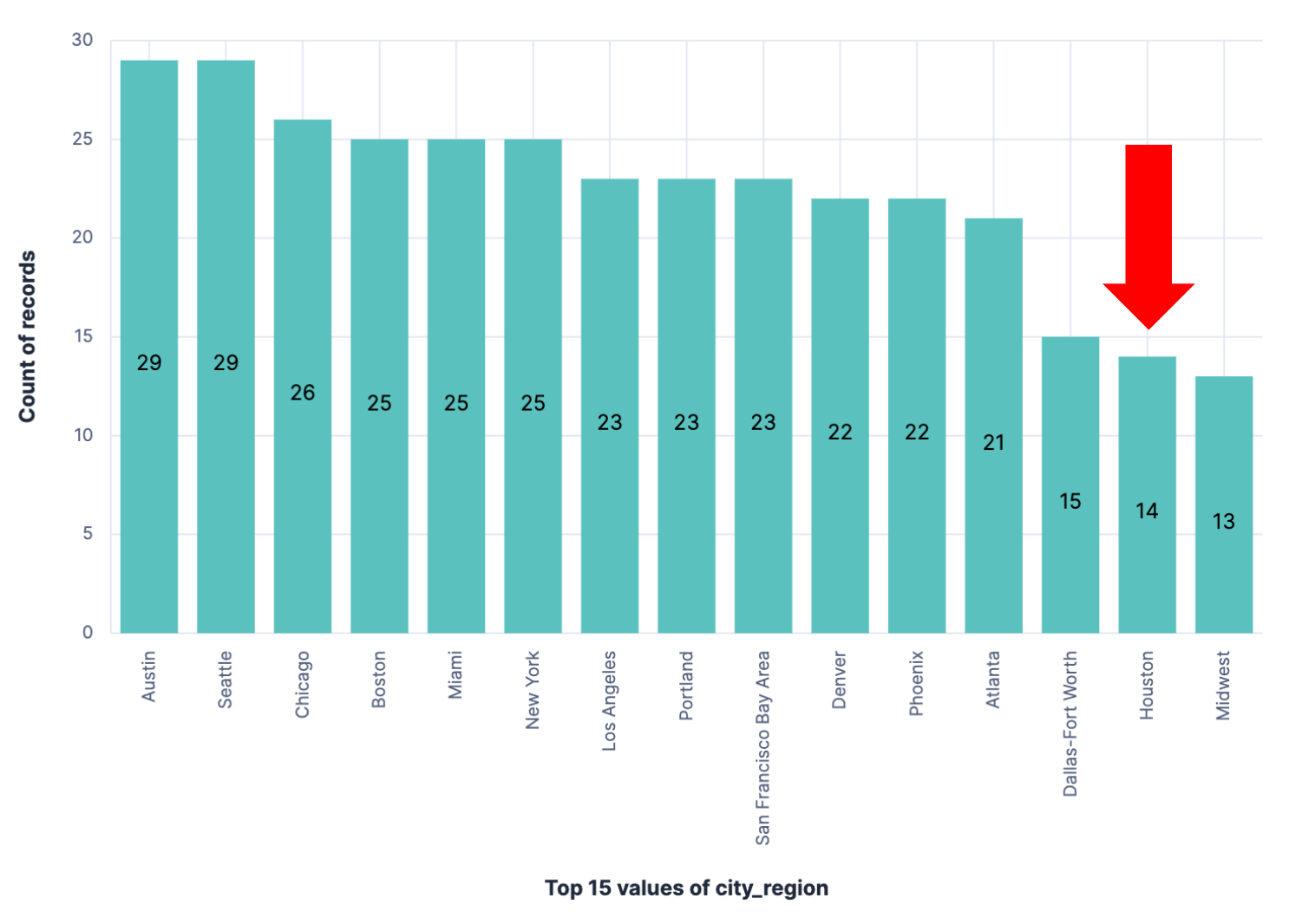
We can see there are 14 sales in Houston, making it the 14th highest city by sales in the dataset.
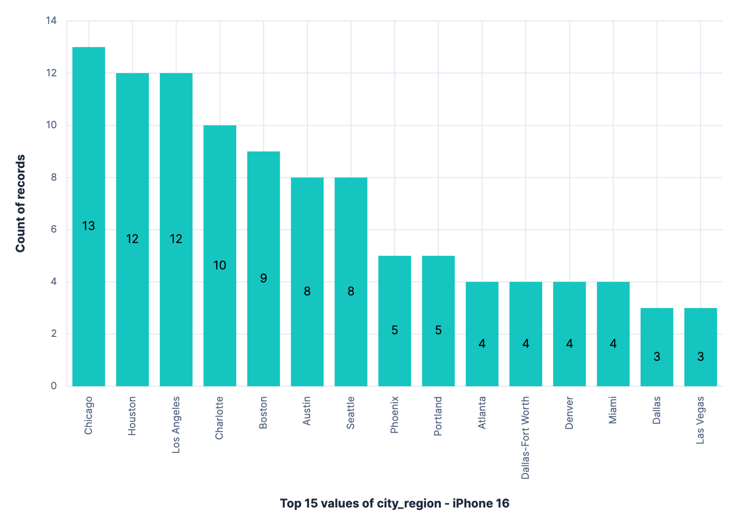
Now, if we apply a filter to look only at the iPhone 16 sales, we have 12 sales in Houston, making it the 2nd city with the most sales for this specific model:
Understanding the significant terms aggregation
According to Elastic documentation, the significant terms aggregation:
”(Finds) terms that have undergone a significant change in popularity measured between a foreground and background set.”
This means it uses statistical metrics to compare the frequency of a term in a subset of data (the foreground set) against the frequency of the same term in the parent set of data (the background set). This way, the scoring reflects statistical significance rather than how often a term appears in the data.
The main differences between a significant terms aggregation and a normal terms aggregation are:
- Significant terms compares a subset of the data, while a terms aggregation only works on the dataset resulting from the query.
- The results from a terms aggregation are the most common terms in the dataset, while the results from a significant terms ignores the common terms to find what makes the dataset unique.
- Significant terms can have a bigger impact on performance, given that it needs to get data from the disk rather than from memory, like the terms aggregation does.
Practical application (consumer behavior analysis)
Preparing data for the analysis
For this analysis, we generated a synthetic phone sales dataset including price, phone specs, demographics of the buyer, and feedback. We also generated embeddings from the user’s feedback to be able to run a semantic query later on. We used the multilingual e5 small model, available out-of-the-box on Elasticsearch.
To use this dataset on Elasticsearch:
- Upload the CSV file (downloadable from here) using the Kibana Upload data files feature.
- Set up a semantic field as shown in this blog called “embedding” that uses the
multilingual-e5-small model - Finish the import with the field type defaults (keyword for every field except for
purchase_dateanduser_feedback). Make sure to add the index namephone_sales_analysisto be able to run the queries presented here as-is.
The main focus of this analysis is to discover "What's different about the iPhone 16 buyers versus other segments of the population?” and to get a segmentation of the buyers for marketing purposes.
This is a sample document from the dataset:
{
         "customer_type": "Returning",
         "user_feedback": "I have to say, quality is great for the price. The battery life is really good.",
         "upgrade_frequency": "2 years",
         "storage_capacity": "256GB",
         "occupation": "Technology & Data",
         "color": "Phantom Black",
         "gender": "Male",
         "price_paid": 899,
         "previous_brand_loyalty": "Mixed",
         "location_type": "Urban",
         "phone_model": "Samsung Galaxy S24",
         "city_region": "San Francisco Bay Area",
         "@timestamp": "2024-03-15T00:00:00.000-05:00",
         "income_bracket": "75000-100000",
         "purchase_channel": "Online",
         "feedback_sentiment": "positive",
         "education_level": "Bachelor",
         "embedding": "I have to say, quality is great for the price. The battery life is really good.",
         "customer_id": "C001",
         "purchase_date": "2024-03-15",
         "age": 34,
         "trade_in_model": "iPhone 13"
}
Understanding demographic patterns
Here, we are going to run an analysis on the general population and compare it to interesting findings from the significant terms aggregations for iPhone 16 users.
Normal patterns
To understand normal buying patterns, we can aggregate data over all documents across different fields. For simplicity, we’ll focus on exploring the occupations of the people who bought a phone. We can do this with a request to Elasticsearch.
GET phone_sales_analysis/_search
{
"aggs": {
"occupation_distribution": {
"terms": {
"size": 5,
"field": "occupation"
}
}
},
"size": 0
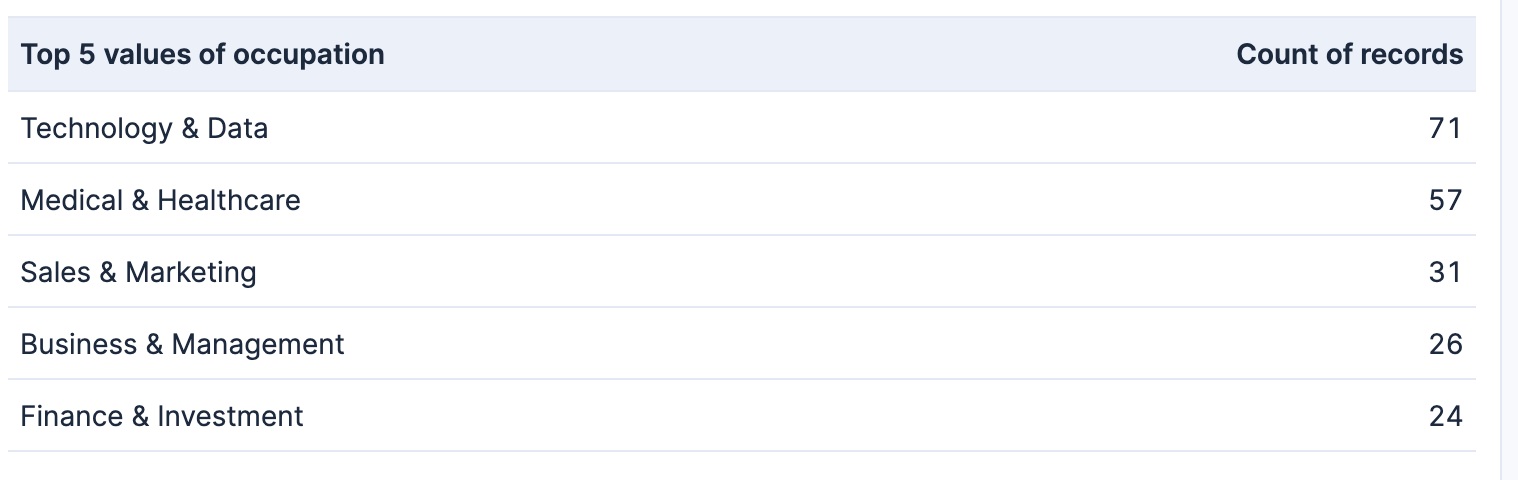
}This tells us that the main occupations in the dataset (by number of records) are:
iPhone 16 users’ patterns
To understand what is different about people who bought an iPhone 16, let’s run a terms aggregation on the same field with a filter to find those people in the query, like this:
GET phone_sales_analysis/_search
{
  "query": {
    "term": {
      "phone_model": "iPhone 16"
    }
  },
  "aggs": {
    "occupation_distribution": {
      "terms": {
        "size": 5,
        "field": "occupation"
      }
    }
  },
  "size": 0
}
So, for iPhone 16 users, the main occupations are:
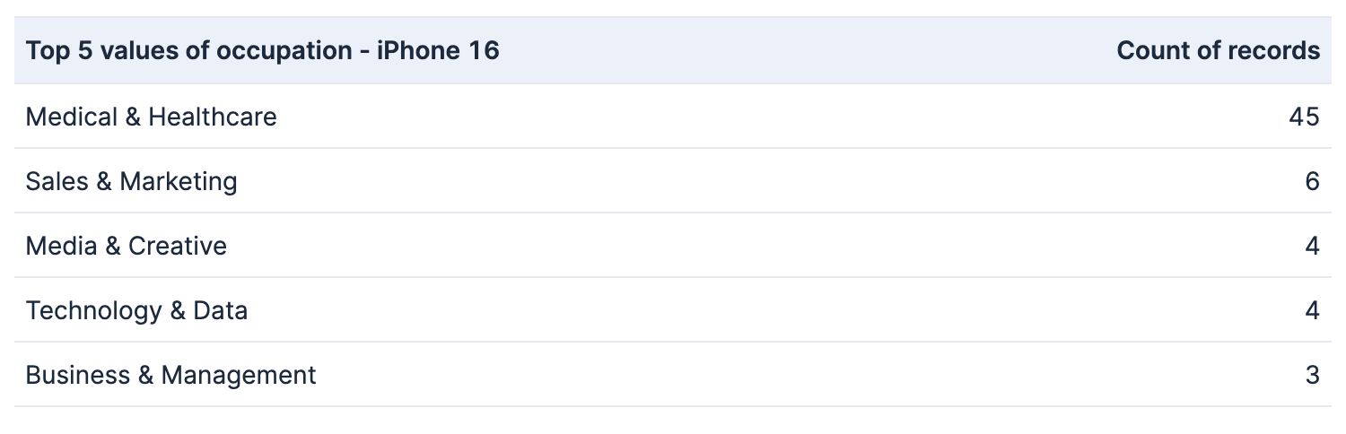
We can see that iPhone 16 users have different occupation patterns compared to users of other phone models. Let’s use Kibana to easily visualize the results:
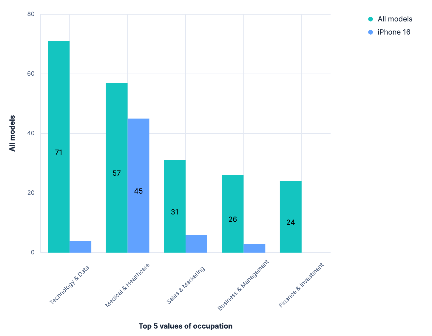
In this chart, we can see that the trend for the iPhone 16 is different from the trend of the whole population.
We can skip this whole analysis to see what makes iPhone 16 users different from the general population by running one significant terms aggregation:
GET phone_sales_analysis/_search
{
  "query": {
    "term": {
      "phone_model": "iPhone 16"
    }
  },
  "aggs": {
    "occupation_distribution": {
      "significant_terms": {
        "size": 5,
        "field": "occupation"
      }
    }
  },
  "size": 0
}
In short, we get this response:
| Values of occupations for the iPhone 16 | doc_count | bg_count |
|---|---|---|
| occupation_distribution (top level) | 122 | 424 |
| Medical & Healthcare bucket | 45 | 57 |
The response clearly suggests that iPhone 16 users have an uncommon (read significant!) number of people in the medical & healthcare field compared to the general population. Let’s see what the numbers in the response mean:
- At the top level:
- doc_count: 122 — The query matched 122 documents total
- bg_count: 424 — The background set (all the sales documents) contains 424 documents
- In the Medical & Healthcare bucket:
- doc_count: 45 — "Medical & Healthcare" appears in 45 of the 122 query results
- bg_count: 57 — "Medical & Healthcare" appears in 57 of the 424 total documents in the background dataset
Out of 424 buyers, 57 work in the medical & healthcare field — or 13.44%. But when we look at the iPhone 16 buyers, 45 out of 122 work in the medical & healthcare field — that is 36.88%. This means we are twice as likely to find someone working in medical & healthcare among iPhone 16 users!
We can apply this same analysis to other fields (age, location, income bracket, etc.) to find more information on what makes iPhone 16 users unique.
Consumer segmentation
We can use the significant terms aggregation to extract relationship insights between products, categories, and customer segments. For this, we build a parent aggregation for the category we are interested in exploring. We also use a significant terms and a normal terms sub-aggregation to find interesting insights on that category and compare them to what most people in that occupation use.
For example, let’s see what people in some work fields prefer:
- To make the analysis clearer, let’s limit our search to 3 work fields: ["Administrative & Support", "Technology & Data", "Medical & Healthcare"]
- On the aggregations side, we start with a terms aggregation by occupation
- Add one subaggregation: terms by phone model—to find which models users who work in each field are buying
- Add a second subaggregation: significant terms by phone models—to find which models are special in each work field
GET phone_sales_analysis/_search
{
 "query": {
   "terms": {
     "occupation": [
       "Administrative & Support",
       "Technology & Data",
       "Medical & Healthcare"
     ]
   }
 },
 "aggs": {
   "occupations": {
     "terms": {
       "size": 15,
       "field": "occupation"
     },
     "aggs": {
       "general_models": {
         "terms": {
           "field": "phone_model"
         }
       },
       "significant_models": {
         "significant_terms": {
           "field": "phone_model"
         }
       }
     }
   }
 },
 "size": 0
}
Let’s break down the aggregation results:
Occupation: Administrative & Support
Terms aggregation
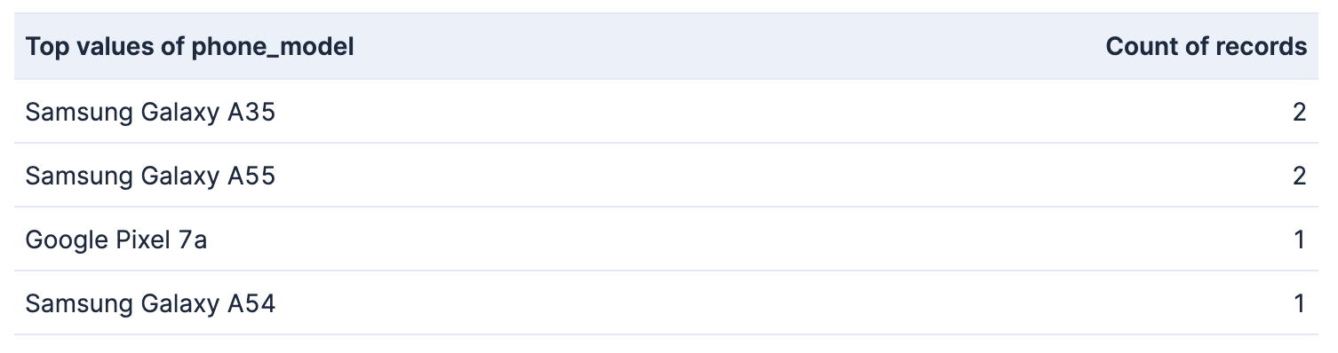
Significant terms aggregation

From this table, we can infer that there are no significant differences between the trend for this occupation and the trend for the entire population
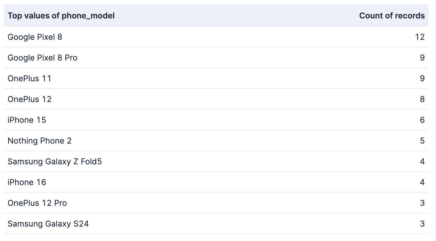
Occupation: Technology & Data
Terms aggregation
Significant terms aggregation
Total documents: 424
Documents in this occupation: 71
| phone model | doc_count (this model in this occupation) | bg_count (this model in all the documents) | % in all the documents | % in this occupation |
|---|---|---|---|---|
| Google Pixel 8 | 12 | 22 | 5.19% | 16.90% |
| OnePlus 11 | 9 | 14 | 3.30% | 12.68% |
| OnePlus 12 Pro | 3 | 3 | 0.71% | 4.23% |
| Google Pixel 8 Pro | 9 | 21 | 4.95% | 12.68% |
| Nothing Phone 2 | 5 | 8 | 1.89% | 7.04% |
| Samsung Galaxy Z Fold5 | 4 | 6 | 1.42% | 5.63% |
| OnePlus 12 | 8 | 20 | 4.72% | 11.27% |
Occupation: Medical & Healthcare
Terms aggregation
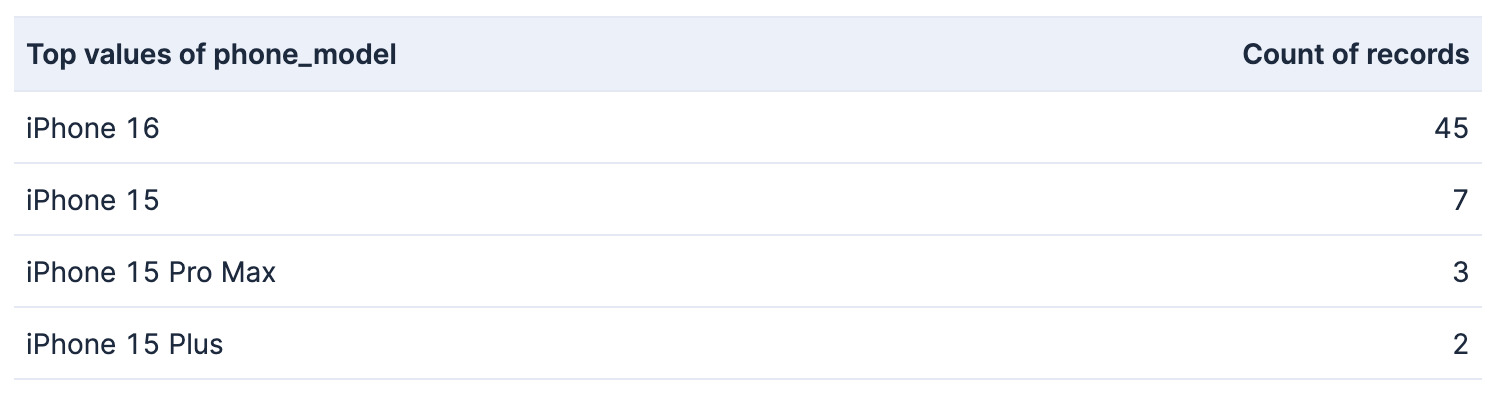
Significant terms aggregation
Total documents: 424
Documents in this occupation: 57
| phone model | doc_count (this model in this occupation) | bg_count (this model in all the documents) | % in all the documents | % in this occupation |
|---|---|---|---|---|
| iPhone 16 | 45 | 122 | 28.77% | 78.95% |
| iPhone 15 Pro Max | 3 | 13 | 3.07% | 5.26% |
| iPhone 15 | 7 | 40 | 9.43% | 12.28% |
Let’s see what story this data is telling us:
- Medical & healthcare professionals prefer the iPhone 16 and are very inclined to use Apple phones in general.
- Technology & data professionals prefer high-end Android phones, but do not necessarily use the Samsung brand. There is also a sizable trend for iPhones in this category.
- Administrative & support professionals prefer Samsung and Google phones, but do not have a strong and unique trend.
Significant terms aggregation and Hybrid search
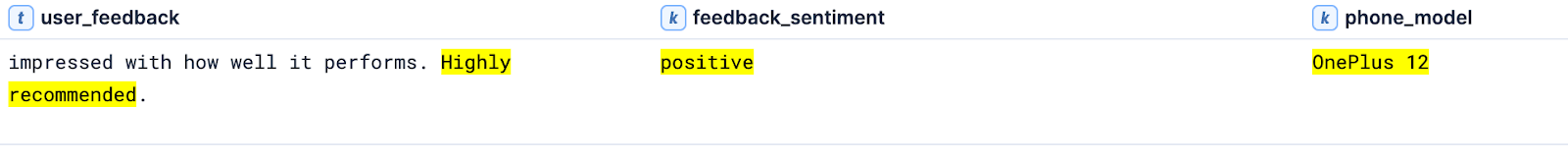
Hybrid search combines text search and semantic results to provide an improved search experience. In this context, a significant term aggregation can provide insights into the results of a context-aware search by answering the question: What is special about this dataset compared to all the documents?To demonstrate this feature, let’s see which models are overrepresented when users talk about good performance:
- Let’s build a semantic query where we find the top user feedback closer to the input “good performance” over the field embedding
- We will also use a text search with the same terms over the text field user_feedback
- We will also add a significant terms query to find phone models that can be found more frequently among these results than in the complete dataset
GET phone_sales_analysis/_search
{
 "retriever": {
   "rrf": {
     "retrievers": [
       {
         "standard": {
           "query": {
             "bool": {
               "must": [
                 {
                   "match": {
                     "user_feedback": {
                       "query": "good performance",
                       "operator": "and"
                     }
                   }
                 }
               ]
             }
           }
         }
       },
       {
         "standard": {
           "query": {
             "semantic": {
               "field": "embedding",
               "query": "good performance"
             }
           }
         }
       }
     ],
    "rank_window_size": 20
   }
 },
 "aggs": {
   "Models": {
     "significant_terms": {
       "field": "phone_model"
     }
   }
 }
}
Let’s look at an example of the matching documents:
This is the response we get:
{
  "took": 388,
  "timed_out": false,
  "_shards": {
    "total": 1,
    "successful": 1,
    "skipped": 0,
    "failed": 0
  },
  "hits": {
    "total": {
      "value": 20,
      "relation": "eq"
    },
    "max_score": 0.016393442,
    "hits": [...]
  },
  "aggregations": {
    "Models": {
      "doc_count": 20,
      "bg_count": 424,
      "buckets": [
        {
          "key": "iPhone 15",
          "doc_count": 5,
          "score": 0.4125,
          "bg_count": 40
        }
      ]
    }
  }
}
This tells us that while an iPhone 15 is encountered 40 times out of 424 total documents (9.4% of the documents), it can be found 5 times in the 20 documents that matched the semantic search “good performance” (25% of the documents). Thus, we can draw a conclusion: an iPhone 15 is 2.7 times more likely to be found when talking about good performance than by chance.
Conclusion
The significant terms aggregation can uncover unique details of a dataset by comparing it to the universe of documents. This can unveil unexpected relationships in our data, going beyond the count of occurrences. We can apply significant terms in various use cases that enable very interesting features, for example:
- Find patterns when working on fraud detection — identify common transactions for stolen credit cards.
- Brand quality insights from user reviews — detect a brand with a disproportionate number of bad reviews.
- Spot misclassified documents — spot documents that belong to a category (term filter) that use uncommon words for the category in a description (significant terms aggregation).
Ready to try this out on your own? Start a free trial.
Want to get Elastic certified? Find out when the next Elasticsearch Engineer training is running!
Related content
October 20, 2025
How to deploy Elasticsearch on an Azure Virtual Machine
Learn how to deploy Elasticsearch on Azure VM with Kibana for full control over your Elasticsearch setup configuration.
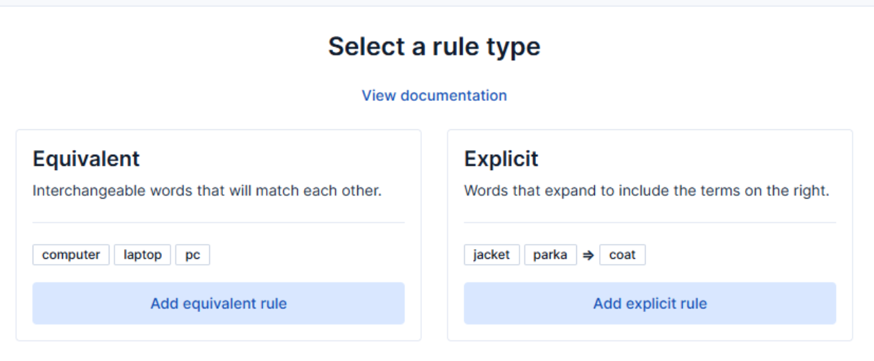
How to use the Synonyms UI to upload and manage Elasticsearch synonyms
Learn how to use the Synonyms UI in Kibana to create synonym sets and assign them to indices.

October 8, 2025
How to reduce the number of shards in an Elasticsearch Cluster
Learn how Elasticsearch shards affect cluster performance in this comprehensive guide, including how to get the shard count, change it from default, and reduce it if needed.
October 3, 2025
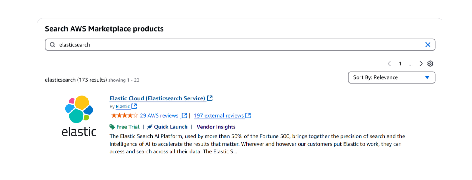
How to deploy Elasticsearch on AWS Marketplace
Learn how to set up and run Elasticsearch using Elastic Cloud Service on AWS Marketplace in this step-by-step guide.

September 29, 2025
HNSW graph: How to improve Elasticsearch performance
Learn how to use the HNSW graph M and ef_construction parameters to improve search performance.