K-means for building vector indices

K-means is a classic clustering algorithm. It prescribes a simple iterative procedure that alternates between assigning vectors to centroids then updating centroids based on their assigned vectors. It is also a critical component of certain classes of vector indexing strategies, specifically a technique called inverted file indexing (IVF).

For IVF indices, vectors are clustered and a map is created which lists the vectors associated with each cluster. Retrieval proceeds by embedding a query, then looking up the nearest cluster centroids and finally comparing the vectors in each cluster to the query vector. This bears a striking resemblance to traditional lexical retrieval by inverted index (hence the name). Compared to graph based methods such as HNSW it has some distinct pros and cons. This post is not intended to survey IVF, which we plan to do elsewhere. Instead we focus on the peculiar characteristics of clustering for IVF and the work we did finding an effective approach.

Motivation

If one considers the retrieval phase of vector IVF, it is clear that it is effectively using a quantized approximation for each vector in initial retrieval: the centroid of the cluster to which it is assigned. It is critical in order to achieve good recall that this quantization retains sufficient information to correctly preserve orderings of distances. Specifically, with high probability one needs

d(q,x_1)<d(q,x_2) \implies d(q,c(x_1))<d(q,c(x_2))

Here, $d(\cdot,\cdot)$ denotes the distance metric, $q$ , $x_1$ and $x_2$ are the query and two corpus embedding vectors, respectively, and $c(\cdot)$ denotes the centroid of a vector’s cluster. The larger the clusters the less likely this is to hold; for example, in the limit there is one cluster for the whole corpus all quantized distances are equal. In fact, to be effective IVF typically picks the number of clusters to control the maximum cluster size. Having fewer than 500 vectors per cluster is standard. This means that the number of clusters $k$ scales linearly with the number of vectors $n$ . Furthermore, the run time of k-means is $\text{O}(nk)$ . This means for IVF conventional k-means scales as $\text{O}(n^2)$ which is not good!

Prior Art

Accelerating k-means

K-means performance has been studied extensively over the years and multiple strategies have been proposed for improving its runtime. The bottleneck comes computing the closest center for each vector.

It is well known that for a sufficiently large random subsample of the data k-means converges to a good approximation of its result on the full dataset. Therefore, a trivial speedup is to simply cluster a random subsample. Typically, the sample size needs to ensure that there are sufficient vectors per cluster. In the context of IVF, this improves constants, but doesn’t tackle quadratic scaling.

For low dimensional data there are data structures, such as k-d trees, which allow one to rule out many non-competitive comparisons. The bounds that these approaches use become ineffective for high dimensional data. However, k-means when applied to data projected onto the largest singular value components often yields similar results to clustering the original dataset. Principal component analysis (PCA) is itself somewhat expensive for high dimensional data being order $\text{O}(nd^2)$ . However, there are efficient randomized approaches for PCA. Putting these pieces together could yield significant performance improvements. However, they do not guarantee subquadratic scaling; they also introduce significant complexity. Furthermore, we’ve previously explored the singular values of embedding models and did not observe rapid decay, so we are not sure they are suitable for this approach.

Finally, there are classes of methods which try to accelerate later iterations of k-means using the observation that clusters rapidly stabilize and relatively few vectors are exchanged in later iterations. These started with the work of Elkan and typically make clever use of the triangle inequality to avoid recomputing cluster assignments for a large proportion of the vectors. These have been shown to be effective for accelerating k-means, even for high dimensional data, when it is run to convergence. However, for IVF it is typically unnecessary to run k-means to convergence. Also Elkan’s method itself is not suitable because it requires quadratic $\text{O}(k^2)$ memory. Variants exist that are more suitable, such as Hamerly’s algorithm, which we explore below. Whilst these can potentially provide a nice practical speed up they do not tackle quadratic complexity.

Building vector indices

Multiple prior works explore recursive clustering approaches for building vector indices. Specifically, SPANN builds clusters recursively until a size constraint is met using a balanced clustering objective. This is close to the initialization procedure we use. However, they target a very large number of clusters: 16% of the full dataset. This forces one to use fast approximate techniques for centroid search even at small scales. It also significantly impacts disk friendliness. Here, we explore cluster sizes in the low hundreds which is typical of VQ-indices such as ScaNN-SOAR.

Breaking the Scaling Barrier

In order to tackle quadratic scaling we somehow need to guarantee that we only ever compare each vector to a $\text{o}(n)$ clusters even if we eventually need $\text{O}(n)$ clusters in total.

There is a very simple strategy which achieves this: cluster the dataset recursively. We pick some maximum cluster count $k_0$ then cluster using $\min(k_0,n/t)$ centroids, where $t$ is the target cluster size. For each cluster that is larger than the target size, simply cluster its assigned vectors using $\min(k_0,n_i/t)$ centroids and repeat.

The first clustering costs $n k_0$ comparisons. If clusterings are fairly balanced, which is a reasonable approximation, we end up $k_0$ clusters each containing roughly $n / k_0$ vectors. Therefore, the next round of clustering costs us roughly $k_0 (n / k_0) k_0$ and so on. The total complexity is

\text{O}\left( n k_0 + k_0 \frac{n}{k_0} k_0 + k_0^2 \frac{n}{k_0^2} k_0 + ... + k_0^p \frac{n}{k_0^p} k_0 \right)

This terminates as soon as a cluster size hits the target $t$ , which is when $n / k_0^p = t$ , so we expect around $p=\log(n/t) / \log(k_0)$ rounds.

Putting all this together we expect complexity to be $\text{O}(n\log(n))$ , which is much more healthy.

The Fix Up

There is a small snag with hierarchical clustering. Vectors are first assigned based on coarse grained structure, which can prevent them winding up in their most appropriate fine grained cluster. This sort of problem is illustrated in the figure below.

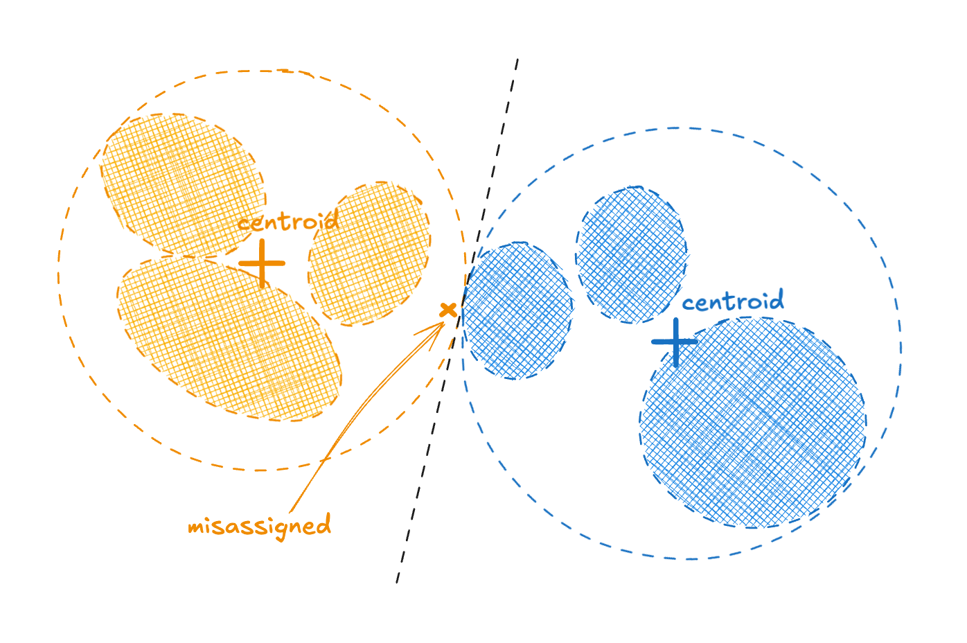
Figure 1 - a problem case for hierarchical clustering

We measured a small increase in within-cluster sum of squares (WCSS) when comparing hierarchical to standard k-means. This translated to a small degradation in index quality and so query recall for the same latency. We wanted to see if we could improve matters whilst not giving up too much of the performance benefits.

We expect that once the recursion has finished the clusters will have stabilized. Specifically, we’ll be in a regime where relatively few vectors need to be exchanged and clusters’ centroids do not change significantly between iterations. In this case, it is sufficient to consider only exchange between a static list of nearest neighbor clusters.

An index of the nearest clusters to each cluster can be built brute force using $\frac{1}{2}k(k-1)$ comparisons. Although this is $\text{O}(n^2)$ comparisons for IVF indices the constants are very good. In particular, if $k$ is around $\frac{n}{500}$ , so this works out as $\frac{1}{500000}n(n-1)$ comparisons. Since we build indices in segments that only reach 10s of millions of vectors this amounts to at most 10s of comparisons per vector. If necessary, fast approximate nearest neighbor schemes can be used at this stage or we can make use of the hierarchy to filter the set of centroids we compare against.

Given the output of hierarchical k-means, standard k-means is then applied, but with each vector considering only a shortlist of $m$ possible clusters on any given iteration.

Spilling with Orthogonality-Amplified Residuals (SOAR)

A recent paper showed nice query performance improvements by allowing each vector to be assigned to multiple clusters. The extra assignments are referred to as spill assignments. To achieve this it makes use of an observation we’ve discussed before: errors parallel to the query vector cost you more than errors perpendicular to the query vector.

Recall that first stage retrieval from an IVF index uses the vector’s cluster centroid as an approximation, for MIP for example the error in this representation is $q^t(x-c(x))$ . Denoting the $i^{\text{th}}$ centroid a vector is assigned to by $c_i(\cdot)$ , SOAR suggests using two assignments and arranging for $x-c_2(x)$ to be approximately perpendicular to $x-c_1(x)$ . This should ensure that at least one of $x-c_1(x)$ or $x-c_2(x)$ is not too parallel to $q$ . This can be done by modifying the assignment objective for computing $c_2$ . For the details see section 3.4 of the paper.

This costs about the same as a single iteration of k-means. Therefore, we explored if we could accelerate spill assignments in exactly the same fashion as our fix up step, using the same shortlist of candidate clusters. We explore the performance of SOAR in the context of our proposed clustering approaches using this acceleration strategy below.

Results

We tested a variety of datasets, distance metrics and embedding vector characteristics. These are summarized in the following table. The datasets comprise a mixture of embedding models and hand engineered features and include both text and image representations.

Dataset	Number vectors	Dimension	Metric
glove 100	1183514	100	Cosine
sift 128	1000000	128	Euclidean
fiqa arctic-base	57638	768	Cosine
fiqa gte-base	57638	768	Cosine
fiqa e5-small	57638	384	Cosine
quora arctic-base	522931	768	Cosine
quora gte-base	522931	768	Cosine
quora e5-small	522931	384	Cosine
gist 960	1000000	960	Euclidean
wiki cohere	934024	768	MIP

We found that Forgy with no restarts was an excellent initialization choice. Indeed, conventionally better initialization schemes like k-means++ actually degrade index quality as measured by query recall for a fixed latency, particularly as it approaches one. We hypothesise that this is because Forgy is properly aligned with our clustering objective. The expected number of centers it places in a region is proportional to the count of vectors it contains. This is exactly what assigning an equal number of vectors per cluster would achieve.

A grid search for $k_0$ , the number of samples to use per cluster and the number of iterations of Lloyd’s algorithm suggests setting them 128, 256 and 12, respectively. These represent a good tradeoff between index quality and build time. All experiments we report use these settings.

In the table below we summarise the raw clustering performance using a target size of $512$ for various alternatives. It shows time to build the index, recall at 3%, cluster size statistics (mean and standard deviation), and the WCSS of the clustering. We report averages over all ten datasets in our test suite. Since the build time and WCSS vary significantly between datasets we normalise them to the k-means result on each dataset. To calculate recall we run with multiple probe counts and measure the recall and number of vector comparisons for each. We interpolate to estimate the average recall achieved when comparing the query to 3% of the dataset.

The methods evaluated are:

k-means: standard k-means using the $n / 512$ clusters.
hierarchical: hierarchical k-means using target cluster size of $512$ .
fix up: hierarchical k-means, using target cluster size of $512$ , followed by fix up with the neighborhood size $m$ equal to $128$ .
Hamerly fix up: uses the same recipe as “fix up” but Hamerly’s variant of k-means is called as a subroutine in hierarchical clustering.

Method	Normalized runtime	Recall @ 3%	Normalized WCSS (lower better)	Cluster size mean	Cluster size standard deviation
k-means	1	0.858	1	512.9	281.5
hierarchical	0.055	0.852	1.015	413.9	152.7
fix up	0.132	0.871	0.991	413.9	153.3
Hamerly fixup	0.132	0.871	0.991	409.7	149.7

In summary, we get a 18 times speedup using hierarchical k-means alone with a drop of 0.6% in recall and an increase of 1.5% in WCSS. With fix up, which roughly doubles the runtime, we still get an 8 times speedup; at the same time we actually get wins in both recall, which increases by 1.3%, and WCSS, which decreases by almost 1%, compared to the baseline. In general, hierarchical approaches undershoot the target cluster size slightly. They also halve the variation in cluster size compared to k-means. This is attractive for IVF search, because it means that the query runtime is more stable for a fixed probe count. We observe that Hamerly doesn’t really provide any benefits given we only run 8 iterations and so is not worth the extra complexity.

Next we turn our attention to SOAR. We studied this using our best baseline clustering approach “fix up”. The main focus was to understand the interaction between the neighborhood size and index quality. We also measured its recall versus latency compared to the baseline.

Our first observation is that of all parameters we explored the one which most consistently affects index quality in the context of SOAR is size of the neighborhood $m$ . If you want to spend build time to improve index quality increase this parameter; however, note it does show diminishing returns. We found the m equal to $128$ achieves nearly optimal quality while still yielding very significant runtime improvements. The overhead computing spill assignments with this choice is around 20% of the total build time. The figures below show the average recall as a function of latency and the relative time to build the index for $m \in \{32,64,128\}$ .

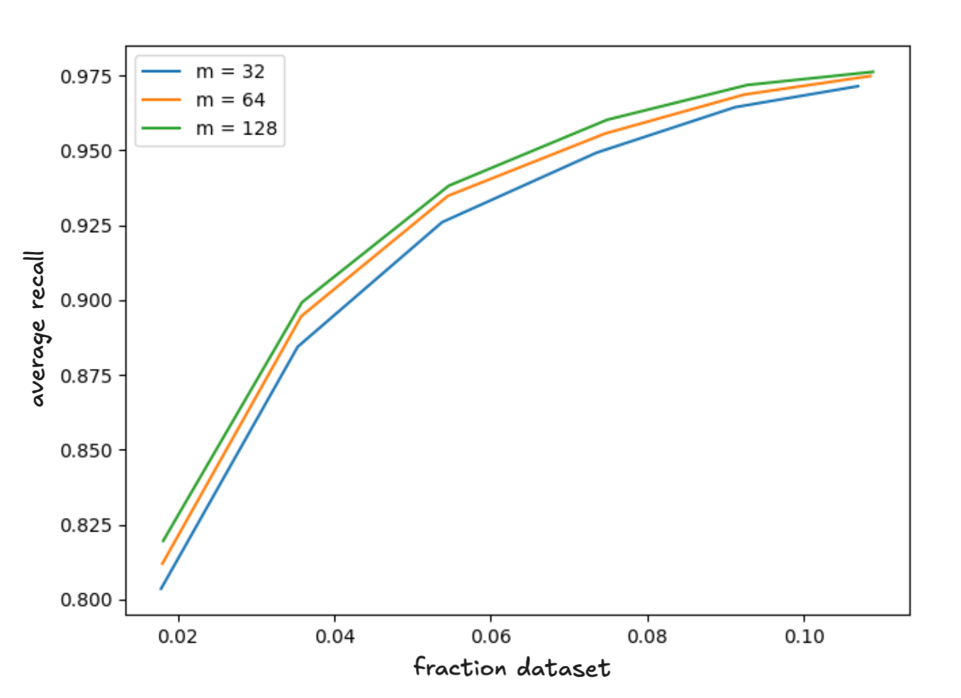
Figure 2 - average recall versus latency for our test suite as a function of the neighborhood size

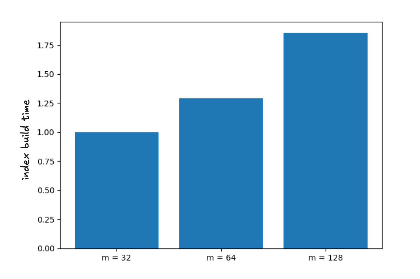
Figure 3 - average build time as a function of neighborhood size normalized to m=32

The figure below shows the average recall versus the number of vector comparisons. We normalize the comparison counts on the X-axis, expressing it as the fraction of the dataset the query is compared to, and average over all ten datasets. Since SOAR nearly doubles cluster sizes we compared to the baseline by retrieving roughly half the number of clusters. In fact, we don’t expect the latency to double because:

We can cache vector comparisons so don’t pay extra cost for any vector that is duplicated in the clusters we compare to the query vector.
We can use fast quantized vector comparisons to extract a subset of candidates to rescore. Rescoring requires relatively expensive floating point vector load and comparison operations that we don’t expect to double with SOAR.

In any case, the graph clearly shows that just measuring latency in terms of vector comparisons SOAR Pareto dominates the baseline achieving better recall at all latencies.

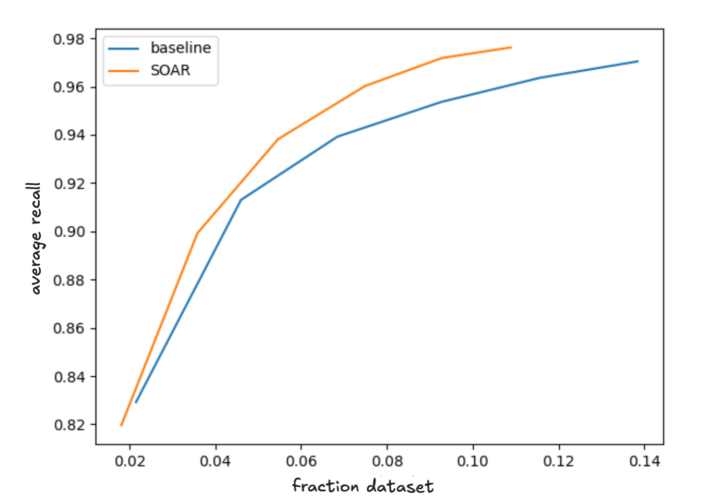
Figure 4 - comparing accelerated SOAR with clustering only

Finally, we discuss how to choose an appropriate value for the target cluster size. For IVF the goal is not to describe the true clusters present in the data, rather to minimize the number of vector comparisons needed to find the nearest neighbors of a query. There is a tradeoff at play: how many centroids you need to compare to find a candidate set of clusters versus how large the candidate set needs to be to achieve a desired recall. In the limit there is one vector per cluster then finding the closest centroid requires you to check every vector in the index, but the recall is always one. In the limit there is one cluster you have to check every vector in the index to resolve the nearest neighbors from that cluster, again the recall is always one. Assuming brute force centroid search, as one increases the target cluster size $t$ the number of centroids to check is $n/t$ , while to achieve acceptable recall $R$ the number of clusters you need to check is some monotonic increasing function $m_R(t)$ . Therefore, the total number of comparisons is $c_R(t)=n/t+m_R(t)t$ . Schematically, this will look something like the following.

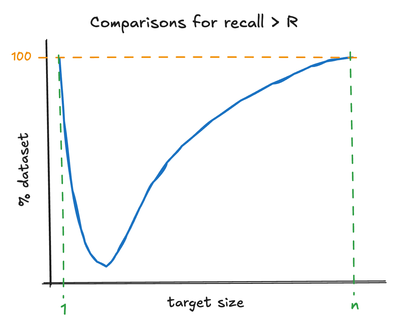
Figure 5 - illustration of IVF index quality as a function of target cluster size (a smaller percentage to achieve recall R is better)

The exact form of $m_R(t)$ depends on the data characteristics and the required recall. The overall query latency will also depend on the centroid search procedure. However, this is only part of the story. Another critical consideration is that cluster size impacts disk friendliness: smaller clusters increase random I/O. Ultimately, optimal query latency will also depend on the memory constraints one operates under.

Since our methods are efficient even for high cluster counts we can explore lower values of target size. In order to maintain acceptable disk friendliness, our expectation is that the optimal cluster sizes will be in the low hundreds and smaller for higher recalls.

In a non-memory constrained setting, we evaluated $t \in \{384,512\}$ . The recall curves are shown below.

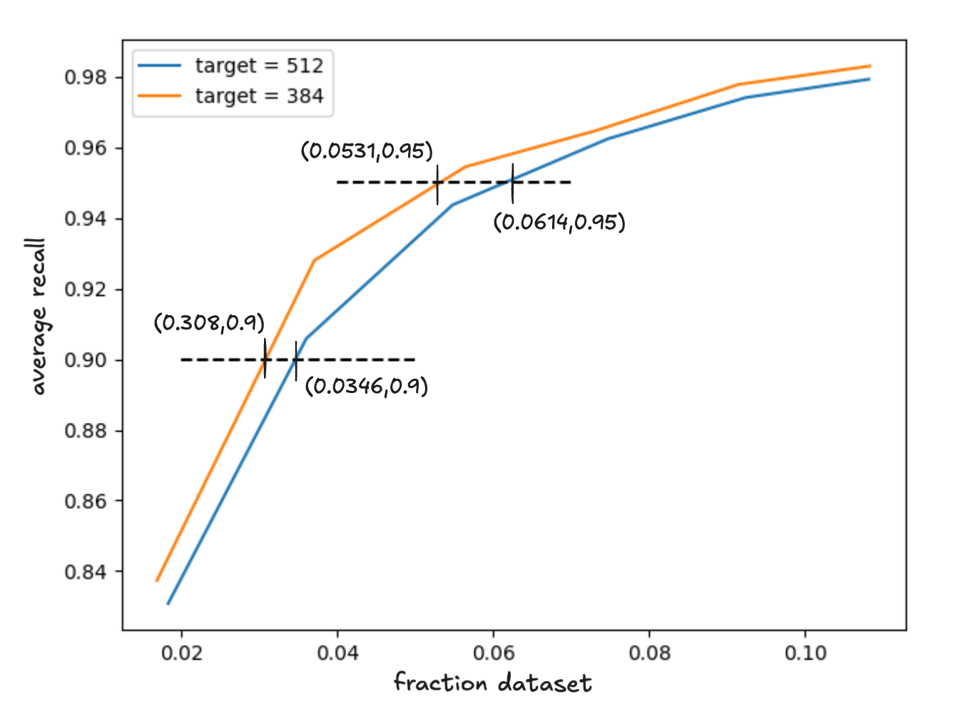
Figure 6 - average recall as a function latency for target cluster sizes 384 and 512

As expected the recall curve for $t=384$ dominates $t=512$ given the candidate set; however, we know that this does not necessarily translate to a net performance improvement because of the cost of finding this set.

For recall $R=0.9$ , $384 \times m_{0.9}(384) / n=0.0308$ and $512 \times m_{0.9}(512) / n=0.0346$ so

\frac{c_{0.9}(384)}{c_{0.9}(512)} \times 100 \%=\frac{(1/384+0.0308)n}{(1/512+0.0346)n} \times 100 \%=94\%

For recall $R=0.95$ , $384 \times m_{0.95}(384) / n=0.0531$ and $512 \times m_{0.95}(512) / n=0.0614$ so

\frac{c_{0.95}(384)}{c_{0.95}(512)} \times 100\%=\frac{(1/384+0.0531)n}{(1/512+0.0614)n} \times 100\%=88\%

In both cases $t=384$ is a net win, by 6% and 12%, respectively. We plan to explore this further in the context of improved centroid search schemes to find a good default target cluster size in our final implementation.

Conclusions

In this post we discussed clustering in the context of the particular constraints imposed by IVF, for which using k-means “as is” has quadratic complexity in the dataset size.

We explored hierarchical k-means to break this scaling and show the resulting scheme requires only $\text{O}(n\log(n))$ comparisons. This results in very substantial speedups: we got an average of 18 times for the datasets in our evaluation set. However, it comes with a small degradation in index quality compared to k-means for cluster sizes in the low hundreds. To address this we introduce a fix up step, allowing for exchange between a subset of cluster pairs. With these changes we achieve an average speedup of 8 times as well as a small improvement in index quality over k-means. We also studied a k-means variant that penalizes creating unbalanced clusterings. This behaves as expected: it creates more uniform clusters and it improves the runtime of hierarchical k-means. However, it slightly degraded index quality in our testing and so we didn’t pursue it further.

We then studied SOAR and showed we were able to achieve recall improvements compared to clustering alone using an accelerated spill assignment scheme. This only considers a subset of clusters as candidates for spill assignments. There is a tradeoff between the index build time and quality since the larger the candidate set size the better the index. We found that using $128$ candidates we achieve most of the benefits whilst still achieving very significant performance improvements.

Finally, we studied how to choose the best target cluster size. We discussed the criteria for selecting the optimal target. To maintain good disk friendliness we expect one will need to use a value in the low hundreds. But there is also considerable scope to improve performance by tuning this parameter. We plan to explore this further offline to identify a good default for Elasticsearch.

Taken together our results show there is substantial scope for improving IVF style index build times and quality by making appropriate choices for the clustering strategy. Although there has been some prior work, there is a large design space and we feel it warrants further exploration.

The work we’ve discussed here will feed into the IVF index implementation we’re bringing to Elasticsearch.

Ready to try this out on your own? Start a free trial.

Elasticsearch has integrations for tools from LangChain, Cohere and more. Join our advanced semantic search webinar to build your next GenAI app!