RAG with a map: Multimodal + geospatial in Elasticsearch

When working with RAG systems, Elasticsearch offers a significant advantage by combining a hybrid search (vector search + traditional text search) approach with hard filters to ensure the retrieved data is relevant to the user query. This makes models less prone to hallucination and, in general, improves your system quality. In this blog, we will explore how we can take a multimodal RAG system to the next level using Elastic’s geospatial search features.

Getting started

You can find the full source code used in this blog here.

Prerequisites

Elasticsearch 8.0.0+
Ollama
- cogito:3b model
Python 3.8+
Python dependencies:
- elasticsearch
- elasticsearch-dsl
- ollama
- clip_processor
  - torch
  - transformers
  - PIL
- streamlit
- json
- os
- typing

Setup

1. Clone the repository:

git clone https://github.com/Alex1795/multimodal_RAG_elasticsearch.git  
cd multimodal_RAG_elasticsearch

2. Install required libraries:

pip install -r requirements.txt

3. Install and set up Ollama:

Download from https://ollama.com/download/

# Download and start the required model
ollama pull cogito:3b
ollama run cogito:3b

4. Configure Elasticsearch

Make sure to have the following environment variables set:
- ES_INDEX
- ES_HOST
- ES_API_KEY
Set the index mapping on Elasticsearch, put special attention to the geolocation and embeddings definition:

PUT mmrag_blog
{  
  "mappings": {  
    "properties": {  
      "title": {  
        "type": "text",  
        "analyzer": "standard"  
      },  
      "geolocation": {  
        "type": "geo_point"  
      },  
      "image_filename": {  
        "type": "keyword"  
      },  
      "generated_description": {  
        "type": "text",  
        "analyzer": "standard"  
      },  
      "description": {  
        "type": "text",  
        "analyzer": "standard"  
      },  
      "text_embedding": {  
        "type": "dense_vector",  
        "dims": 512,  
        "index": true,  
        "similarity": "cosine"  
      },  
      "image_embedding": {  
        "type": "dense_vector",  
        "dims": 512,  
        "index": true,  
        "similarity": "cosine"  
      },  
      "photo_id": {  
        "type": "keyword"  
      }  
    }  
  }  
}

Run the application

1. Generate and index images’ embeddings and metadata:

python upload_documents.py

This file runs the data indexing pipeline. It processes the image metadata files and enriches them with multimodal embeddings (from the description and the image itself using the CLIP model). Finally, it uploads the documents to Elasticsearch. After executing this command, you should see the mmrag_blog index in Elasticsearch with the image metadata, geolocation, and image and text embeddings.

2. Run the streamlit app and use the UI in your browser with:

streamlit run streamlit_app.py #comment

After executing this command, you can see the project webpage at http://localhost:8501.

The webpage is the interface for the RAG application. From there, you can ask a question, and then the assistant will extract the appropriate parameters from your question, run an RRF search on Elasticsearch to find related pictures, and formulate a response. It will also show some pictures from the results.

Implementation overview

To demonstrate Elastic’s RAG capabilities, we will build an assistant that can answer questions about national parks using relevant data. The search combines 4 approaches with data inferred from the user’s text query:

Image vector search
Text vector search
Lexical text search
Geospatial filtering

This allows our assistant to answer questions that are relevant and focused on what the user needs.

Now, how can the geospatial filter improve the assistant results? For example, if the user asks, “Where can I find canyons near Salt Lake City?” Without a geospatial filter, the assistant might suggest:

Canyonlands National Park - Utah
Grand Canyon National Park - Arizona

However, since we know the user is specifically looking for sites near Salt Lake City, it makes sense to look for answers in Utah. Therefore, the correct option is Canyonlands National Park only.

The implementation in this blog uses a geo_distance query to be able to find results (the picture’s geopoint) in a particular national park area. We are also using geoshapes to draw the parks’ areas.

However, Elastic capabilities with geo queries go well beyond that:

geo_bounding_box query: Finds documents (geopoints or geoshapes) that intersect a specified rectangle
geo_grid query: Finds documents that intersect a specified geohash, map tile, or H3 bin
geo_shape query: Finds documents that are related (intersects, is contained by, is within, or a disjoint operation) to the specified geoshape

Dataset

We will use geotagged pictures from national parks obtained from Flickr. We augment these pictures with a description and vectorize both the image and description using the openai/clip-vit-base-patch32 model:

We merge these embeddings with the images’ metadata, and at the end, we get a document that looks like this:

{
         "title": "Spa Geyser in Yellowstone National Park on a sunny day",
         "geolocation": {
           "lat": 44.45899722222222,
           "lon": -110.82573611111111
         },
         "image_filename": "52631363114_Spa_Geyser_in_Yellowstone_National_Park_on_a_sunny.jpg",
         "generated_description": "A small geyser releases steady streams of hot water and steam into the air on a clear sunny day. Colorful mineral deposits surround the thermal feature, creating vibrant orange and yellow formations. The active geothermal vent demonstrates the underground volcanic activity that powers these natural fountains.",
         "text_embedding": [
           0.02323250286281109,
           …
           -0.17811810970306396
         ],
         "image_embedding": [
           -0.22548234462738037,
		…
		-0.040389999747276306
         ]

       }

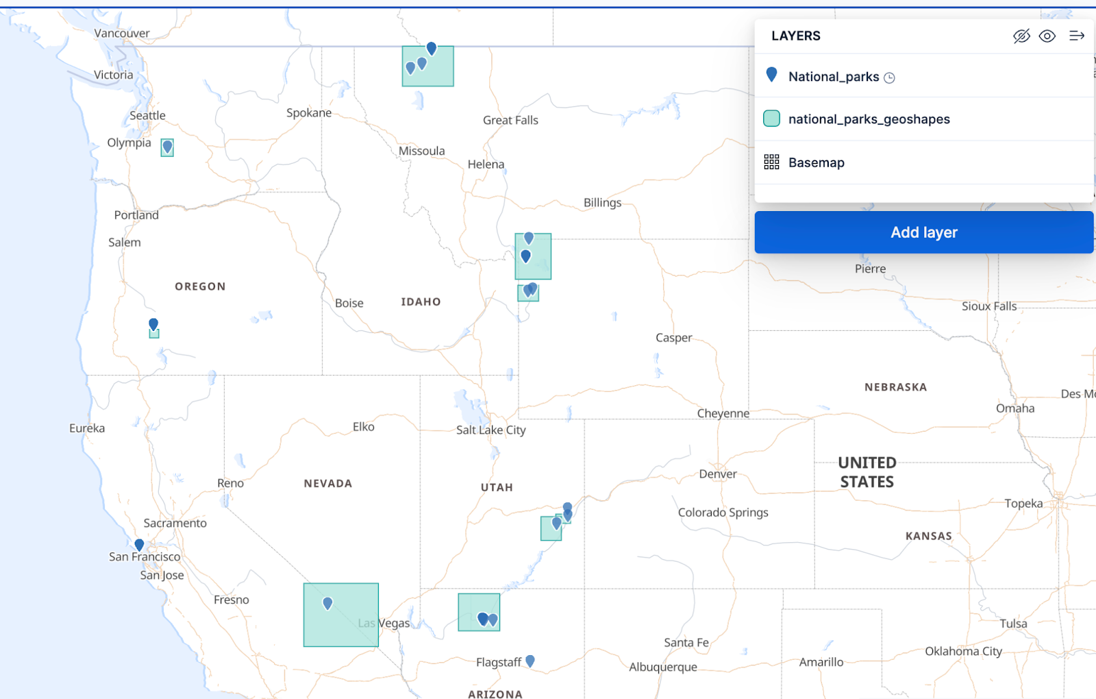
A key benefit of using Elastic with geo positions is the Kibana Maps visualization. In Kibana, our dataset looks like this (note that we also added geo shapes for the national parks):

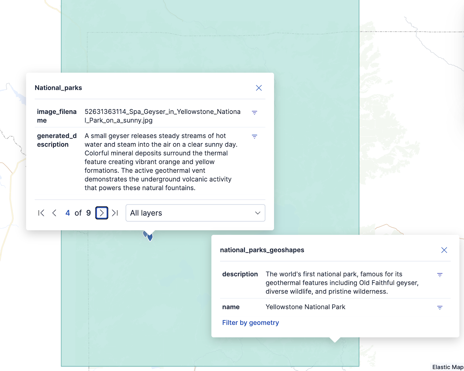
Zooming in, we can see the same document as before in Yellowstone. Additionally, Yellowstone Park’s (approximate) shape is also drawn in the layer below.

System architecture

Indexing pipeline

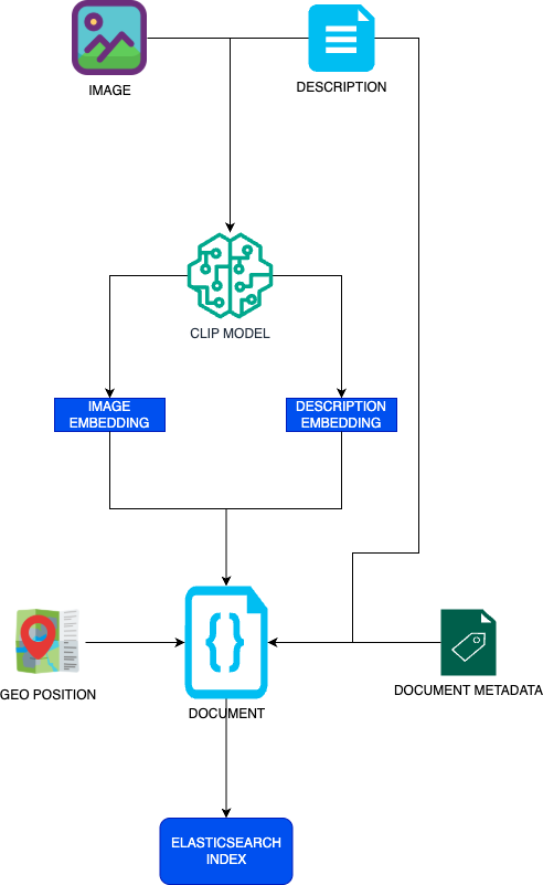
The indexing pipeline will handle the vectorization of both the image and description. It will also add more metadata to the image to create a document and index it to Elastic:

1. The starting point is pairs of images and metadata from national parks. This metadata includes the geolocation, title of the image, and a description.

2. We feed the image and description to the CLIP model (openai/clip-vit-base-patch32) to obtain an embedding of each in the same vectorial space of 512 dimensions. You can see the complete source code of this step here.

def create_image_embedding(image_path):
    image = Image.open(image_path).convert('RGB')
    inputs = processor(images=image, return_tensors="pt", padding=True, truncation=True, use_fast=True)
    with torch.no_grad():
        outputs = model.get_image_features(**inputs)
    return outputs.numpy().flatten()

The process to generate an embedding from our image is:

Load the image in RGB format using Image.open()
Process the image by converting it into tensors, which is the format the model expects, using processor()
Extracts a dense vector representation in 512 dimensions from the image using model.get_image_features()
At the end, converts the PyTorch tensor into a flattened numpy array using outputs.numpy().flatten()

def create_text_embedding(text):
    # Process the text
    inputs = processor(text=[text],  return_tensors="pt", padding=True, truncation=True)
    # Generate embedding
    with torch.no_grad():
        text_features = model.get_text_features(**inputs)
        # Normalize the embedding (CLIP embeddings are typically normalized)
        text_features = text_features / text_features.norm(dim=-1, keepdim=True)
    # Convert to numpy array
    embedding = text_features.numpy().flatten()

    return embedding

The process to generate an embedding from text is:

Processes the input text, tokenizing it and converting it to tensors using processor()
Parses the tokenized text using the model to extract its semantic features using model.get_text_features(). The resulting embedding also has 512 dimensions.
Normalizes the embedding so the dot similarity can be computed using text_features / text_features.norm()
Finally, it converts the embedding into a flattened numpy array using text_features.numpy().flatten()

We chose this model because it is a multimodal model that maximizes the similarity between image and text. This way, a description of an image and the image itself tend to generate embeddings that are close in the vector space.

3. We merge all the metadata, the description, geoposition, and embeddings from the image and description in a JSON file

We index the JSON file to Elastic using:

es.index(document=doc, index=index)

Where doc is the metadata for each image.

Search pipeline

This stage will handle the user’s query, create the search, and generate a response from the search results. The LLM used is cogito:3b with Ollama, though it could be easily replaced by any remote model—like Claude or ChatGPT. We chose this particular model because it’s lightweight and it excels at general tasks (as is expected from an assistant) compared to similar models (like Llama 3.2 3B). This means we get proper results without a long waiting time, and everything is running locally!

The pipeline works like this:

1. We receive an input from the user: Where can I see mountains in Washington State?.

2. We feed the user input and a dictionary of the parks, including their states and geolocations (defined in the same Python file), to the LLM with instructions to extract parameters for the Elastic query. The exact prompt is:

”””You are going to extract data from a user query for a national parks search system. 

Available National Parks:
{parks_info}

Extract the following information and format it as JSON:
- context_search: the main activity or interest (e.g., "hike","walk dog"," or"camping")
- distance_km: estimated search radius in kilometers (default: 100 if not specified)
- location_type: specific state, city, or region mentioned
- reference_location: if a city is mentioned, include it (e.g., "Boston","Denver")
- relevant_parks: list of park IDs that might be relevant based on location (use the exact park IDs from the list above)

Examples:
User query: "Where can I hike in Utah?"
Response: {{"context_search": "hike", "distance_km": 100, "location_type": "Utah", "reference_location": null, "relevant_parks": ["arches_national_park", "canyonlands_national_park"]}}

Only respond with valid JSON. No additional text. If a city is mentioned, use the state that city is in as the location_type.

User query: {query}”””

And this is an example of data in the parks_info dictionary:

 { 
    "mt_rainier_national_park": {
        "coordinates": (46.8523, -121.7603),
        "state": "Washington"
    }
  }

The model extracts the following data from the prompt above:

{
 'context_search': 'mountains', 
 'distance_km': 100, 
 'location_type': 'Washington', 
 'reference_location': None, 
 'relevant_parks': ['mt_rainier_national_park']
}

3. We use the context_search parameter to generate a new embedding using the same CLIP model.

4. We extract the coordinates from the parks_info dictionary.

5. We use all these parameters to create an Elasticsearch query. This is the heart of the RAG feature:

We create a geo_distance filter using the coordinates and the 'distance_km' parameter.
We create a match text query against the ‘generated_description’ field.
We create a standard retriever that uses the text query from the previous step and the geo_distance filter.
We create two knn retrievers that use the embedding created in step 4 and match it against the image embedding and text embedding indexed on each document. Each retriever also uses the geo_distance filter.
We use an RRF retriever to combine the resulting datasets of all the other retrievers.

This whole process is executed in the rrf_search() function:

def rrf_search(index_name, lat, lon, distance, text_query, k=10,
               num_candidates=100):
    """
    Create an RRF search object bound to a specific index. Then executes the search. 

    Args:
        index_name (str): Name of the Elasticsearch index
        lat (float): Latitude for geo filtering
        lon (float): Longitude for geo filtering
        distance (int/str): Distance for geo filtering
        text_query (str): Text to search in description fields
        k (int): Number of top results for KNN search
        num_candidates (int): Number of candidates for KNN search

    Returns:
        Search: List of results frm Elasticsearch
    """

    embedding = create_text_embedding(text_query).tolist()

    # Create geo distance query
    geo_filter = Q('geo_distance',
                   distance=distance,
                   geolocation={'lat': lat, 'lon': lon})

    # Create text search queries
    text_queries = [
        Q('match', generated_description=text_query),
        Q('match', description=text_query)
    ]

    # Create boolean query for standard search
    standard_query = Q('bool', filter=[geo_filter], should=text_queries)

    # Create search object bound to index
    s = Search(index=index_name)
    s = s.source(["image_filename", "generated_description"])
    # Build RRF configuration
    retrievers = [
        # Standard retriever
        {
            "standard": {
                "query": standard_query.to_dict()
            }
        },
        # Text KNN retriever
        {
            "knn": {
                "filter": geo_filter.to_dict(),
                "field": "text_embedding",
                "query_vector": embedding,
                "k": k,
                "num_candidates": num_candidates
            }
        },
        # Image KNN retriever
        {
            "knn": {
                "filter": geo_filter.to_dict(),
                "field": "image_embedding",
                "query_vector": embedding,
                "k": k,
                "num_candidates": num_candidates
            }
        }
    ]

    # Apply RRF configuration
    s = s.extra(retriever={'rrf': {'retrievers': retrievers}}, size=3)

    #print(s.to_dict())

    es = Elasticsearch(cloud_id=cloud_id, api_key=api_key)

    results = s.using(es).execute()["hits"]["hits"]

    return results

At the end, we obtain a query like this:

{
 "retriever": {
   "rrf": {
     "retrievers": [
       {
         "standard": {
           "query": {
             "bool": {
               "filter": [
                 {
                   "geo_distance": {
                     "distance": "100km",
                     "geolocation": {
                       "lat": 46.8523,
                       "lon": -121.7603
                     }
                   }
                 }
               ],
               "should": [
                 {
                   "match": {
                     "generated_description": "mountains"
                   }
                 }
               ]
             }
           }
         }
       },
       {
         "knn": {
           "filter": {
             "geo_distance": {
               "distance": "100km",
               "geolocation": {
                 "lat": 46.8523,
                 "lon": -121.7603
               }
             }
           },
           "field": "text_embedding",
           "query_vector": [
             0.01967986486852169,
             ...
             0.00988344382494688],
           "k": 10,
           "num_candidates": 100
         }
       },
       {
         "knn": {
           "filter": {
             "geo_distance": {
               "distance": "100km",
               "geolocation": {
                 "lat": 46.8523,
                 "lon": -121.7603
               }
             }
           },
           "field": "image_embedding",
           "query_vector": [
             0.01967986486852169,
             ...
             0.00988344382494688],
           "k": 10,
           "num_candidates": 100
         }
       }
     ]
   }
 },
 "size": 3,
 "_source": [
   "image_filename",
   "generated_description"
 ]
}

6. Afterwards, we feed the documents obtained from Elastic and the user’s original query to the LLM with this prompt:

f"""You are a helpful assistant for national parks activities. Based on the search results below, provide a comprehensive and helpful response to the user's original query.

Original User Query: {original_query}

Search Parameters Used:
- Activity/Interest: {search_params.get('context_search', 'N/A')}
- Search Distance: {search_params.get('distance_km', 'N/A')} km
- Location: {search_params.get('location_type', 'N/A')}

Search results: {results_text}

Instructions:
- Provide a natural, conversational response
- Recommend specific activities and locations based on the search results only
- Include practical information when available
- Do not suggest alternatives if no results were found
- Be enthusiastic and helpful about national parks experiences
- Keep the response focused and not too lengthy
- Structure your response separating your suggestions per national park
- Do not include anything about national parks that are not in the results"""

7. Finally, the LLM creates a response from the search results:

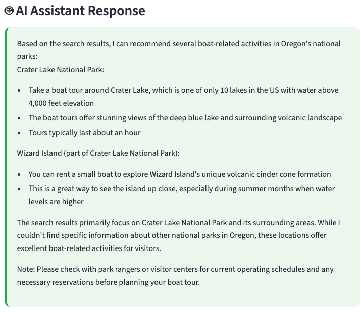
I'd be happy to help you find mountains in Washington State! Based on the search results, here are some fantastic locations:
Mount Rainier National Park is a must-visit destination for mountain lovers. Paradise Valley offers breathtaking views of the Tatoosh Mountain Range and Mount Rainier itself. The best time to visit is during late spring when the wildflowers bloom.

This location offers incredible opportunities to see mountains up close and personal - whether you're hiking, camping, or simply taking in the breathtaking scenery. Would you like more specific information about this park?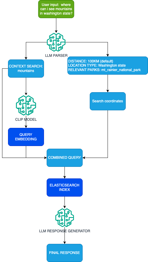

Web application

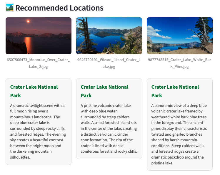
A front-end based on Streamlit handles the user input, runs the search pipeline to obtain the LLM final response, and displays images from the search results with their descriptions.

You can find the application source code and instructions here.

Multimodal RAG and geospatial search usage example

Query: Any places to ride a boat in Oregon?

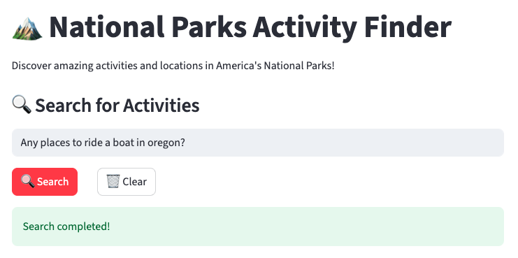
Here, the LLM extracted these parameters:

{
 'context_search': 'boat ride', 
 'distance_km': 100, 
 'location_type': 'Oregon', 
 'reference_location': None, 
 'relevant_parks': ['crater_lake_national_park']
}

And the search centered on Crater Lake National Park, so the response comes only from this national park in Oregon. This way, the system makes sure that it responds to the user under the given constraints and does not mention other parks where a boat ride is possible, but are not in Oregon.

Conclusion

In this article, we saw how integrating multimodal RAG capabilities with Elasticsearch's robust geospatial features significantly enhances the relevance and accuracy of search results in RAG systems. By combining image and text vector search with lexical search and precise geo-filtering, the system can provide highly contextualized answers. This approach not only minimizes hallucinations but also leverages Elasticsearch's diverse geo-query options and Kibana's visualization tools to deliver a comprehensive and user-centric search experience.

Ready to try this out on your own? Start a free trial.

Want to get Elastic certified? Find out when the next Elasticsearch Engineer training is running!