In this blog, we will discuss how to implement a scalable data processing pipeline using NVIDIA NeMo Retriever extraction models, Unstructured Platform and Elasticsearch. This pipeline transforms unstructured data from a data source into structured, searchable content ready for downstream AI applications, such as RAG. Retrieval Augmented Generation (RAG) is an AI technique where Large Language Models (LLMs) are provided with external knowledge to generate responses to user queries. This allows LLM responses to be tailored to specific context, making answers more accurate and relevant.
Before we get started, let’s take a look at the key components enabling this pipeline and what each brings to the table.
Pipeline components
NeMo Retriever extraction is a set of microservices for transforming unstructured documents into structured content and metadata. It handles document parsing, visual structure identification, and OCR processing at scale. The RAG NVIDIA AI Blueprint provides a starting point for how to use the NeMo Retriever microservices in a high-performance extraction pipeline.
Unstructured is an ETL+ platform for orchestrating the entirety of unstructured data processing: from ingesting unstructured data from multiple data sources, converting raw, unstructured files into structured data through a configurable workflow engine, enriching data with additional transformations, all the way to uploading the results into vector stores, databases and search engines. It provides a visual UI, APIs, and scalable backend infrastructure to orchestrate document parsing, enrichment, and embedding in a single workflow.
Elasticsearch is an industry-leading search and analytics engine that now includes native vector search capabilities. It can function as both a traditional text database and a vector database, enabling semantic search at scale with features like k-NN similarity search.
Now that we’ve introduced the core components, let’s take a look at how they work together in a typical workflow before diving into the implementation.
RAG with NeMo Retriever - Unstructured - Elasticsearch
While here we only provide key highlights, you can find the full notebook here.
This blog can be divided into 3 parts:
- Setting up the source and destination connectors
- Setting up the workflow with Unstructured API
- RAG over the processed data
Unstructured workflow is represented as a DAG where the nodes, called connectors, control where the data is ingested from and where the processed results are uploaded to. These nodes are required in any workflow. A source connector configures ingestion of the raw data from a data source, and the destination connector configures the data uploading of the processed data into a vector store, search engine, or a database.
For this blog, we store research papers in Amazon S3 and we want the processed data to be delivered into Elasticsearch for downstream use. This means that before we can build a data processing workflow, we need to create a source connector for Amazon S3, and a destination connector for Elasticsearch with Unstructured API.
Step 1: Setting up the S3 source connector
When creating a source connector, you need to give it a unique name, specify its type (e.g. S3, or Google Drive), and provide the configuration which typically contains the location of the source you're connecting to (e.g. S3 bucket URI, or Google Drive folder) and authentication details.
source_connector_response = unstructured_client.sources.create_source(
    request=CreateSourceRequest(
        create_source_connector=CreateSourceConnector(
            name="demo_source1",
            type=SourceConnectorType.S3,
            config=S3SourceConnectorConfigInput(
                key=os.environ['S3_AWS_KEY'],
                secret=os.environ['S3_AWS_SECRET'],
                remote_url=os.environ["S3_REMOTE_URL"],
                recursive=False #True/False
            )
        )
    )
)

pretty_print_model(source_connector_response.source_connector_information)
Step 2: Setting up the Elasticsearch destination connector
Next, let’s set up the Elasticsearch destination connector. The Elasticsearch index that you use must have a schema that is compatible with the schema of the documents that Unstructured produces for you—you can find all the details in the documentation.
destination_connector_response = unstructured_client.destinations.create_destination(
    request=CreateDestinationRequest(
        create_destination_connector=CreateDestinationConnector(
            name="demo_dest-3",
            type=DestinationConnectorType.ELASTICSEARCH,
            config=ElasticsearchConnectorConfigInput(
                hosts=[os.environ['es_host']],
                es_api_key=os.environ['es_api_key'],
                index_name="demo-index"
            )
        )
    )
)
Step 3: Creating a workflow with Unstructured
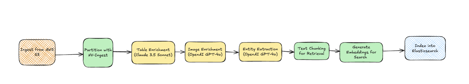
Once you have the source and destination connectors, you can create a new data processing workflow. We’ll build the workflow DAG with the following nodes:
- NeMo Retriever for document partitioning
- Unstructured’s Image Summarizer, Table Summarizer, and Named Entity Recognition nodes for content enrichment
- Chunker and Embedder nodes for making the content ready for similarity search
from unstructured_client.models.shared import (
    WorkflowNode,
    WorkflowNodeType,
    WorkflowType,
    Schedule
)

# Partition the content by using NV-Ingest
parition_node = WorkflowNode(
            name="Ingest",
            subtype="nvingest",
            type="partition",
            settings={"nvingest_host":  userdata.get('NV-Ingest-host-address')},
        )


# Summarize each detected image.
image_summarizer_node = WorkflowNode(
    name="Image summarizer",
    subtype="openai_image_description",
    type=WorkflowNodeType.PROMPTER,
    settings={}
)

# Summarize each detected table.
table_summarizer_node = WorkflowNode(
    name="Table summarizer",
    subtype="anthropic_table_description",
    type=WorkflowNodeType.PROMPTER,
    settings={}
)

# Label each recognized named entity.
named_entity_recognizer_node = WorkflowNode(
    name="Named entity recognizer",
    subtype="openai_ner",
    type=WorkflowNodeType.PROMPTER,
    settings={
        "prompt_interface_overrides": None
    }
)

# Chunk the partitioned content.
chunk_node = WorkflowNode(
    name="Chunker",
    subtype="chunk_by_title",
    type=WorkflowNodeType.CHUNK,
    settings={
        "unstructured_api_url": None,
        "unstructured_api_key": None,
        "multipage_sections": False,
        "combine_text_under_n_chars": 0,
        "include_orig_elements": True,
        "max_characters": 1537,
        "overlap": 160,
        "overlap_all": False,
        "contextual_chunking_strategy": None
    }
)

# Generate vector embeddings.
embed_node = WorkflowNode(
    name="Embedder",
    subtype="azure_openai",
    type=WorkflowNodeType.EMBED,
    settings={
        "model_name": "text-embedding-3-large"
    }
)


response = unstructured_client.workflows.create_workflow(
    request={
        "create_workflow": {
            "name": f"s3-to-es-NV-Ingest-custom-workflow",
            "source_id": source_connector_response.source_connector_information.id,
            "destination_id": "a72838a4-bb72-4e93-972d-22dc0403ae9e",
            "workflow_type": WorkflowType.CUSTOM,
            "workflow_nodes": [
                parition_node,
                image_summarizer_node,
                table_summarizer_node,
                named_entity_recognizer_node,
                chunk_node,
                embed_node
            ],
        }
    }
)

workflow_id = response.workflow_information.id
pretty_print_model(response.workflow_information)

job = unstructured_client.workflows.run_workflow(
    request={
        "workflow_id": workflow_id,
    }
)

pretty_print_model(job.job_information)
Once your job for this workflow completes, the data is uploaded into Elasticsearch and we can proceed with building a basic RAG application.
Step 4: RAG setup
Let's go ahead with a simple retriever that will connect to the data, take in the user query, embed it with the same model that was used to embed the original data, and calculate cosine similarity to retrieve the top 3 documents.
from langchain_elasticsearch import ElasticsearchStore
from langchain.embeddings import OpenAIEmbeddings
import os

embeddings = OpenAIEmbeddings(
    model="text-embedding-3-large",
    openai_api_key=os.environ['OPENAI_API_KEY']

)

vector_store = ElasticsearchStore(
    es_url=os.environ['es_host'],
    index_name="demo-index",
    embedding=embeddings,
    es_api_key=os.environ['es_api_key'],
    query_field="text",
    vector_query_field="embeddings",
    distance_strategy="COSINE"
)

retriever = vector_store.as_retriever(
    search_type="similarity",
    search_kwargs={"k": 3}  # Number of results to return
)
Then let's set up a workflow to receive a user query, fetch similar documents from Elasticsearch, and use the documents as context to answer the user’s question.
from openai import OpenAI

client = OpenAI(api_key=os.getenv("OPENAI_API_KEY"))

def generate_answer(question: str, documents: str):

    prompt = """
    You are an assistant that can answer user questions given provided context.
    Your answer should be thorough and technical.
    If you don't know the answer, or no documents are provided, say 'I do not have enough context to answer the question.'
    """

    augmented_prompt = (
        f"{prompt}"
        f"User question: {question}\n\n"
        f"{documents}"
    )
    response = client.chat.completions.create(
        messages=[
            {'role': 'system', 'content': 'You answer users questions.'},
            {'role': 'user', 'content': augmented_prompt},
        ],
        model="gpt-4o-2024-11-20",
        temperature=0,
    )

    return response.choices[0].message.content


def format_docs(docs):
    seen_texts = set()
    useful_content = [doc.page_content for doc in docs]

    return  "\nRetrieved documents:\n" + "".join(
        [
            f"\n\n===== Document {str(i)} =====\n" + doc
            for i, doc in enumerate(useful_content)
        ]
    )
def rag(query):
  docs = retriever.invoke(query)
  documents = format_docs(docs)
  answer = generate_answer(query, documents)
  return documents, answer
Putting everything together we get:
query = "How did the response lengths change with training?"

docs, answer = rag(query)

print(answer)
And a response:
Based on the provided context, the response lengths during training for the DeepSeek-R1-Zero model showed a clear trend of increasing as the number of training steps progressed. This is evident from the graphs described in Document 0 and Document 1, which both depict the "average length per response" on the y-axis and training steps on the x-axis.

### Key Observations:
1. **Increasing Trend**: The average response length consistently increased as training steps advanced. This suggests that the model naturally learned to allocate more "thinking time" (i.e., generate longer responses) as it improved its reasoning capabilities during the reinforcement learning (RL) process.

2. **Variability**: Both graphs include a shaded area around the average response length, indicating some variability in response lengths during training. However, the overall trend remained upward.

3. **Quantitative Range**: The y-axis for response length ranged from 0 to 12,000 tokens, and the graphs show a steady increase in the average response length over the course of training, though specific numerical values at different steps are not provided in the descriptions.

### Implications:
The increase in response length aligns with the model's goal of solving reasoning tasks more effectively. Longer responses likely reflect the model's ability to provide more detailed and comprehensive reasoning, which is critical for tasks requiring complex problem-solving.

In summary, the response lengths increased during training, indicating that the model adapted to allocate more resources (in terms of response length) to improve its reasoning performance.
Elasticsearch provides various strategies to enhance search, including Hybrid search, a combination of approximate semantic search and keyword-based search.
This approach can improve the relevance of the top documents used as context in the RAG architecture. To enable it, you need to modify the vector_store initialization as follows:
from langchain_elasticsearch import DenseVectorStrategy

vector_store = ElasticsearchStore(
    es_url=os.environ['es_host'],
    index_name="demo-index",
    embedding=embeddings,
    es_api_key=os.environ['es_api_key'],
    query_field="text",
    vector_query_field="embeddings",
    strategy=DenseVectorStrategy(hybrid=True) // <-- here the change
)
Conclusion
Good RAG starts with well-prepared data, and Unstructured simplifies this critical first step. By enabling partitioning with NeMo Retriever, metadata enrichment of unstructured data and efficient ingestion into Elasticsearch, it ensures that your RAG pipeline is built on a solid foundation, unlocking its full potential for all your downstream tasks.
Ready to try this out on your own? Start a free trial.
Elasticsearch has integrations for tools from LangChain, Cohere and more. Join our advanced semantic search webinar to build your next GenAI app!
Related content
June 16, 2025
Elasticsearch open inference API adds support for IBM watsonx.ai rerank models
Exploring how to use IBM watsonx™ reranking when building search experiences in the Elasticsearch vector database.
June 13, 2025
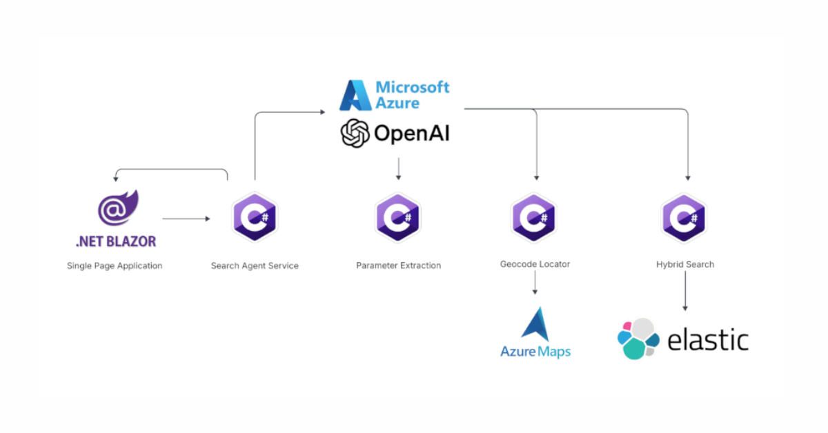
Using Azure LLM Functions with Elasticsearch for smarter query experiences
Try out the example real estate search app that uses Azure Gen AI LLM Functions with Elasticsearch to provide flexible hybrid search results. See step-by-step how to configure and run the example app in GitHub Codespaces.
June 17, 2025
Improving Copilot capabilities using Elasticsearch
Discover how to use Elasticsearch with Microsoft 365 Copilot Chat and Copilot in Microsoft Teams.
June 5, 2025
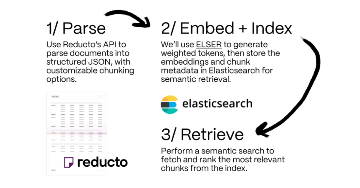
Making sense of unstructured documents: Using Reducto parsing with Elasticsearch
Demonstrating how Reducto's document processing can be integrated with Elasticsearch for semantic search.

May 21, 2025
First to hybrid search: with Elasticsearch and Semantic Kernel
Hybrid search capabilities are now available in the .NET Elasticsearch Semantic Kernel connector. Learn how to get started in this blog post.