Last year, we described how you can use ES|QL to perform geospatial search, and followed up with a blog on ingesting geospatial data for use in ES|QL. While these blogs introduced the powerful geospatial search capabilities in ES|QL, they did not cover one of the most desired features, distance search, introduced into ES|QL in Elasticsearch 8.15.
As with all the geospatial features we've been adding to ES|QL, this feature was designed to conform closely to the Simple Feature Access standard from the Open Geospatial Consortium (OGC) and it is used by other spatial databases like PostGIS, making it much easier to use for GIS experts familiar with these standards.
In this blog, we'll show you how to use ES|QL to perform geospatial distance searches and how it compares to the SQL and Query DSL equivalents.
Searching for geospatial data
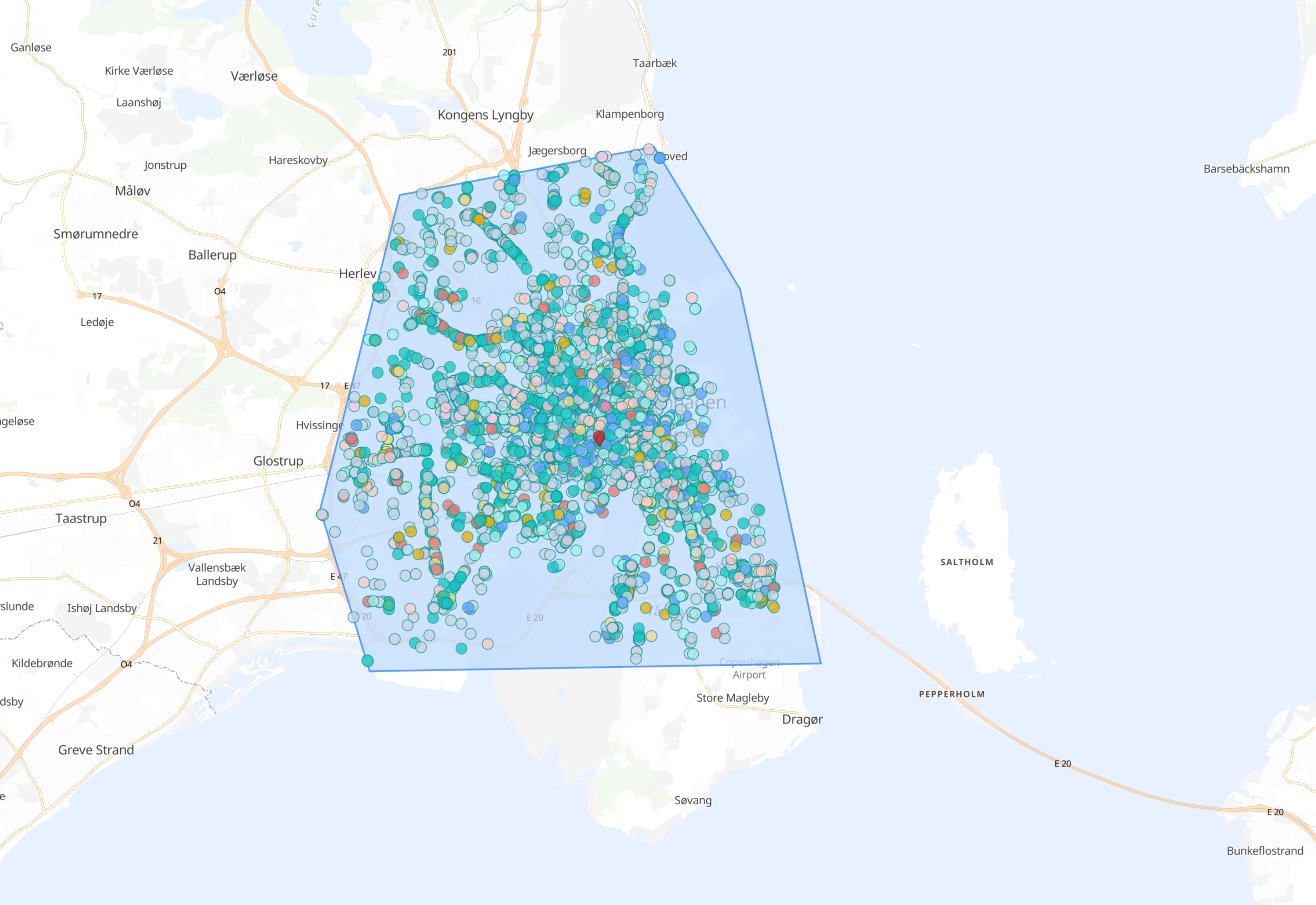
Let's remind ourselves of the main search function we used in the previous blog, the ST_INTERSECTS function. Assuming you have a dataset of points of interest (POIs) in Denmark, such as the Geofabrik download of OpenStreetMap Data for Denmark, and have imported it into Elasticsearch (for example, by using Kibana map's ability to import ESRI ShapeFiles), you can use ES|QL to search for points of interest within a specific area, in this case, the city of Copenhagen:
FROM denmark_pois
| WHERE name IS NOT NULL
| WHERE ST_INTERSECTS(
    geometry,
    TO_GEOSHAPE(
      "POLYGON ((12.444077 55.606669, 12.681656 55.608996, 12.639084 55.720149, 12.593765 55.762282, 12.459869 55.747985, 12.417984 55.654735, 12.444077 55.606669))"
    )
  )
| LIMIT 10000
This performs a search for any point geometry within the simple polygon we used to outline the city of Copenhagen.
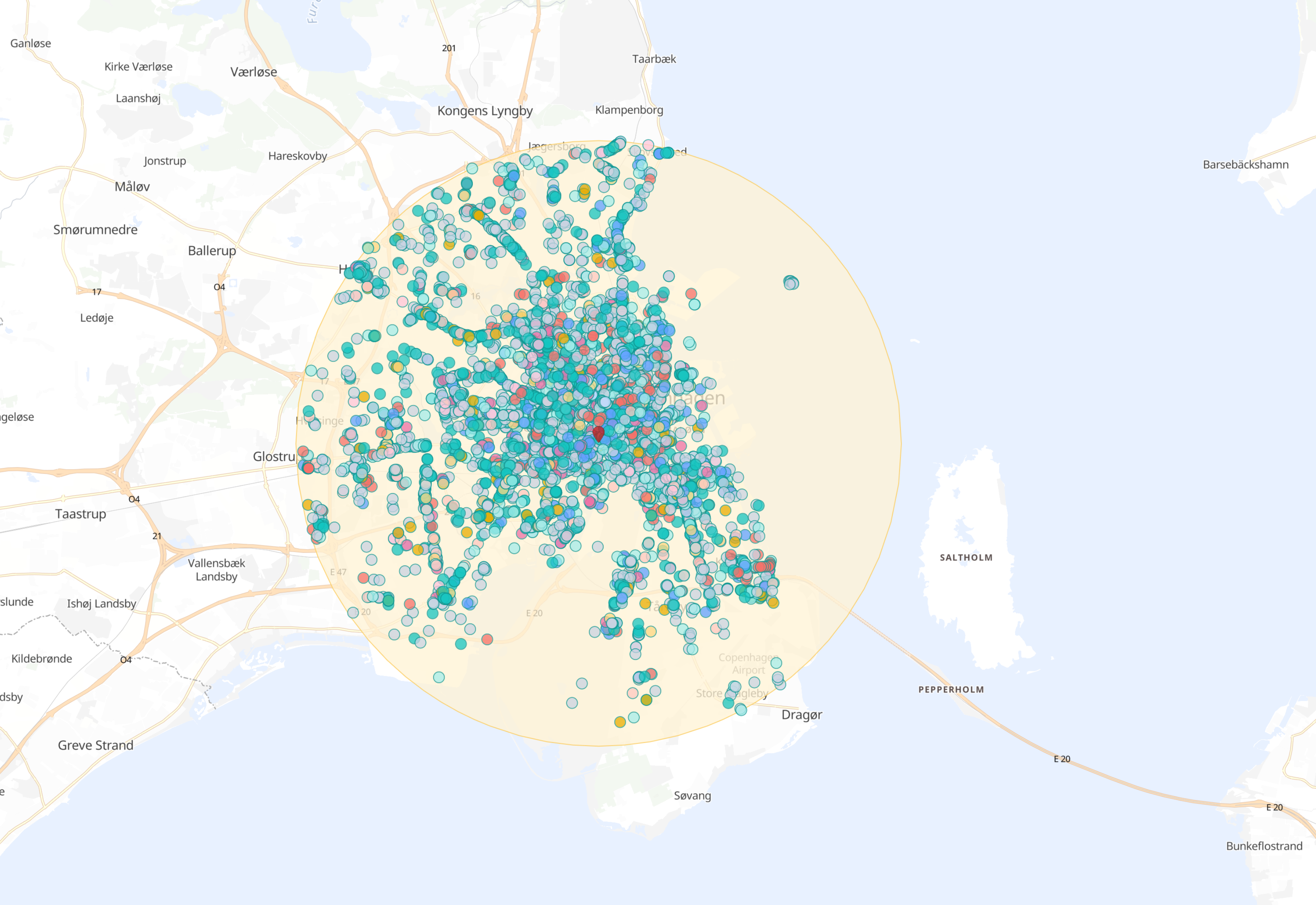
But the query was not particularly pretty with that large polygon expression. What we are far more likely to want to ask is for all points within a distance of a central point, perhaps our current location at the Copenhagen Central Train Station:
FROM denmark_pois
| WHERE name IS NOT NULL
| WHERE ST_DISTANCE(
    geometry,
    TO_GEOPOINT("POINT (12.564926 55.672938)")
  ) < 10000
| LIMIT 10000
This much simpler query asks for all points within 10,000 meters (10 km) of the point at latitude 55.672938 and longitude 12.564926, inside the central station.
Now, compare this to the equivalent query in the Elasticsearch Query DSL:
POST denmark_pois/_search
{
  "size": 10000,
  "query": {
    "geo_distance": {
      "distance": "10km",
      "geometry": {
        "lat": 55.672938,
        "lon": 12.564926
      }
    }
  }
}
Both queries are reasonably clear in their intent. However, notice that the ES|QL query closely resembles SQL. The same query in PostGIS looks like this:
SELECT *
FROM denmark_pois
WHERE ST_Distance(
    geometry::geography,
    ST_SetSRID(ST_MakePoint(12.564926, 55.672938), 4326)::geography
) < 10000
LIMIT 10000;
Look back at the ES|QL example. So similar, right? In fact, the ES|QL query is even simpler than the PostGIS query as it does not require the ST_SetSRID function to set the coordinate reference system (CRS) of the point geometry. Nor does it require the ::geography type-cast to ensure the distance calculation is done on a spherical coordinate system. This is because the ES|QL function TO_GEOPOINT uses the geo_point type, which is always in the WGS84 CRS, and also ensures all distance calculations are done on a spherical coordinate system.
The distance calculation
This leads to an important question: how does the distance calculation work? As mentioned above, the ES|QL geo_point type is always in the WGS84 coordinate reference system (CRS), which is a spherical CRS. The actual calculation of the distance is done using the Haversine formula, which calculates the distance between two points on a sphere given their latitude and longitude. This is done for both the ES|QL ST_DISTANCE function and the Query DSL geo_distance query.
This leads to another important point. Since we are compatible with the Query DSL, and can even make use of the same underlying Lucene spatial index, the distance calculation is also restricted to the same precision as defined in the Lucene spatial index. Lucene uses a quantization function to convert 64-bit floating point numbers to 32-bit integers, which means that all spatial functions in Elasticsearch, and therefore in ES|QL too, are limited to this precision, of the order of 1cm. Read more about this in this blog: BKD-backed geo_shapes in Elasticsearch: precision + efficiency + speed.
Other uses of ST_DISTANCE
We can use the ST_DISTANCE function in many other ways, including when the results are not intended for display on a map:
FROM denmark_pois
| WHERE name IS NOT NULL
| WHERE ST_DISTANCE(geometry, TO_GEOPOINT("POINT (12.564926 55.672938)")) < 10000
| STATS count=COUNT() BY fclass
| SORT count DESC
| LIMIT 16
Results in a table of the number of 'points of interest' for category, sorted by the most common category:
count | fclass
---------------+---------------
1528 |fast_food
930 |cafe
842 |restaurant
492 |clothes
490 |bar
457 |hairdresser
368 |artwork
364 |supermarket
326 |convenience
258 |bakery
255 |bicycle_shop
184 |kiosk
135 |beverages
133 |jeweller
120 |butcher
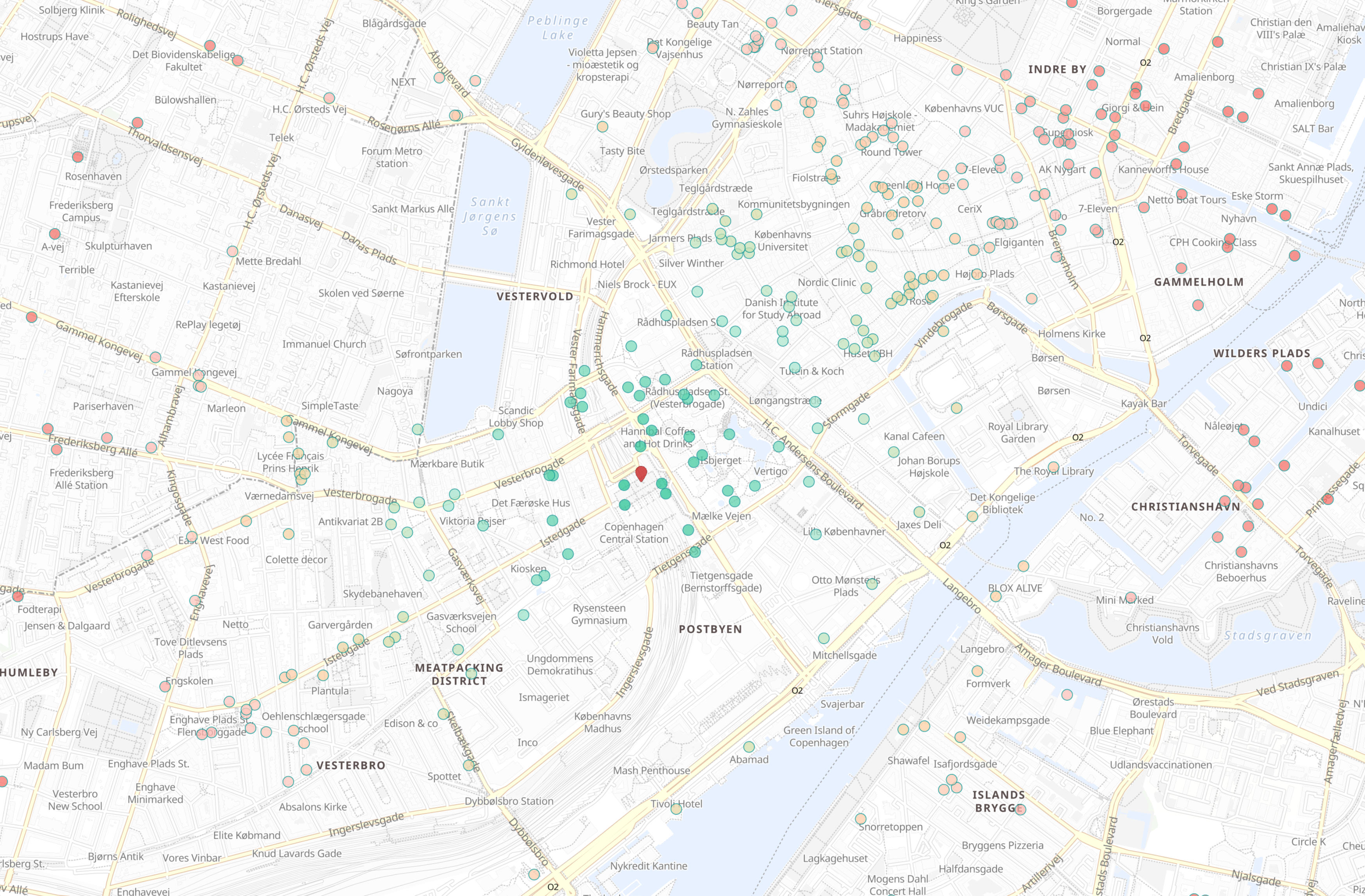
113 |pubSo next we might want to focus on Cafés and find the closest ones to the central station:
FROM denmark_pois
| WHERE name IS NOT NULL AND fclass == "cafe"
| EVAL distance = ST_DISTANCE(geometry, TO_GEOPOINT("POINT (12.564926 55.672938)"))
| WHERE distance < 2000
| SORT distance ASC
| LIMIT 100
This query not only filters the results to only include Cafés, but calculates and returns the distance, with the closest Cafés sorted first. We can even use the reported distances to color the map in Kibana:
Why not SQL?
What about Elasticsearch SQL? It has been around for a while and has some geospatial features. However, Elasticsearch SQL was written as a wrapper on top of the original Query API, which meant only queries that could be transpiled down to the original API were supported. ES|QL does not have this limitation. Being a completely new stack allows for many optimizations that were not possible in SQL. It even allows for features not possible in the Query API, such as the EVAL command, which allows you to evaluate expressions and return results. Our benchmarks show ES|QL is very often faster than the Query API, particularly with aggregations!
Clearly, from the earlier examples, ES|QL is quite similar to SQL, but there are some important differences, which we discussed in much more detail in the earlier blog on Geospatial search in ES|QL.
ST_DISTANCE performance
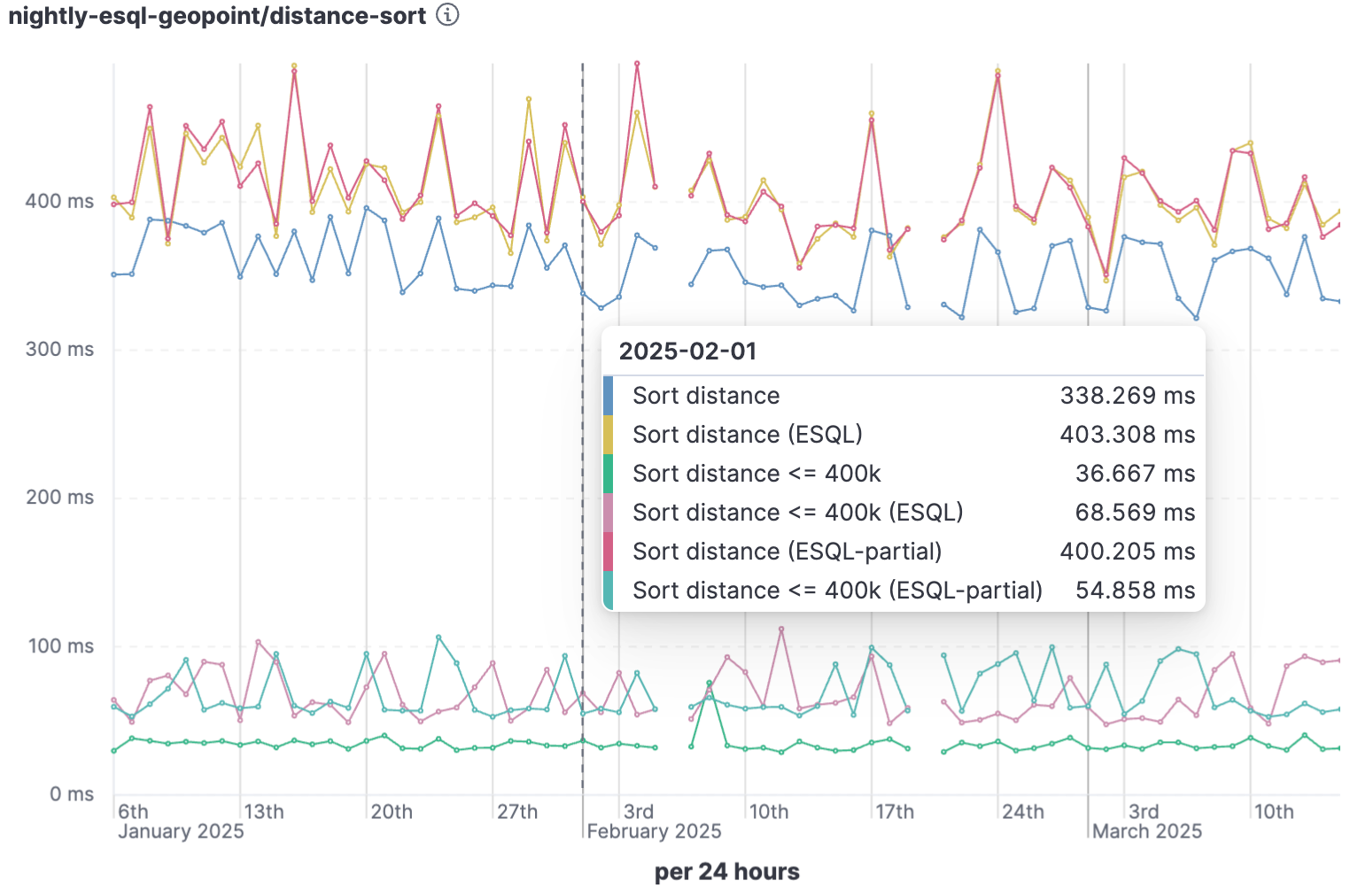
An obvious question is how does the ST_DISTANCE function perform? At first glance, it seems like it would be slow, as it requires calculating the distance for every point in the index. However, this is not the case. The ST_DISTANCE function is optimized to use the same spatial index as the geo_distance query in the Query DSL. In fact, even the SORT distance ASC command is optimized to use the same spatial index, so it is very fast.
Last year, when we first implemented the ST_DISTANCE function, it took about 30s to run on our benchmarking dataset. Then we performed an optimization called 'Lucene Pushdown' whereby we make sure that appropriate queries make optimal use of the underlying Lucene index when possible, and after that, the same query took only 50ms.
So, how are these optimizations achieved? In general, with declarative query languages like ES|QL, the query engine can analyze the query and determine the best way to execute it. Whether a function like ST_DISTANCE can be optimized depends on the query structure and the underlying data. Consider the following query:
FROM airports
| EVAL distance = ST_DISTANCE(location, TO_GEOPOINT("POINT(12.565 55.673)"))
| WHERE distance < 1000000 AND scalerank < 6 AND distance > 10000
| SORT distance ASC
| KEEP distance, abbrev, name, location, country, city
This query calculates the distance from Copenhagen Central Station to all airports, filters the results to only include important airports (scalerank less than 6), and a distance between 10km and 1000km, which rules out Copenhagen Airport itself, and sorts the results by distance. That's quite a lot of work to do. How can we make this fast? Well, the query engine contains a set of rules, each of which performs a specific optimization. Applying the rules repeatedly to the query can iteratively transform the query into a semantically equivalent query that is much, much faster.
In the case of our example, the following changes were made:
- A
LIMIT 1000was added at the end (something ES|QL always does if you don't add one yourself). - The
SORTandLIMITwere merged into a singleTOPNcommand, which is something Lucene has special support for. - The
WHEREclause was split into two parts, one that filters by distance and another that filters byscalerank, so that the refined process would become:- Filter first by
scalerank, a known index field, easy to optimize with 'Lucene Pushdown'. - Calculate the distance only for the remaining documents, which is a much smaller set.
- Filter by distance (both the lower and upper bounds), which might also be amenable to later optimization.
- Filter first by
- Finally,
pushdowneverything that can be pushed down to Lucene:- Push the
scalerankfilter down to Lucene - Convert the distance filter into two spatial intersection filters:
ST_INTERSECTS(location, TO_GEOSHAPE("CIRCLE(12.565 55.673, 1000000)"))ST_DISJOINT(location, TO_GEOSHAPE("CIRCLE(12.565 55.673, 10000)"))
- Push these down to Lucene as well, which will use the spatial index to quickly filter out documents that do not match the criteria.
- Push down the
TOPNcommand to Lucene, which has native support forGeoDistanceSort
- Push the
This would dramatically reduce the number of documents returned by the search, leaving much less work for the ES|QL compute engine to perform. Then, the filtered documents would be processed as follows:
- Extract the
locationfield from the remaining documents. - Calculate the distance for each document (since the query was still expected to return values for the
distance). - Extract the other fields requested in the
KEEPcommand. - Send data from all data nodes back to the coordinating node.
- Perform a final sort by distance on the combined results on the coordinating node.
As mentioned above, the performance of queries like this is impressive. In our benchmarks, it took only 50ms to run on a dataset of 60 million points, compared to 30s when no index optimizations were applied.
OGC Functions
As described in the previous blog, Elasticsearch 8.14 introduced four OGC spatial search functions. With the addition of ST_DISTANCE in 8.15, we now have a complete set of OGC functions that we consider part of the core "Spatial Search" functions in ES|QL:
- ST_INTERSECTS: Returns true if two geometries intersect, and false otherwise. Compare this to ST_Intersects in PostGIS.
- ST_DISJOINT: Returns true if two geometries do not intersect, and false otherwise. The inverse of
ST_INTERSECTS. Compare this to ST_Disjoint in PostGIS. - ST_CONTAINS: Returns true if one geometry contains another, and false otherwise. Compare this to ST_Contains in PostGIS.
- ST_WITHIN: Returns true if one geometry is within another, and false otherwise. The inverse of
ST_CONTAINS. Compare this to ST_Within in PostGIS. - ST_DISTANCE: Returns the distance between two geometries. If the field type is
geo_point, the distance is calculated using spherical calculations, the same as the existing Elasticsearch geo_distance query. Compare this to ST_Distance in PostGIS.
All these functions behave similarly to their PostGIS counterparts, and are used in the same way. If you follow the documentation links in the text above, you might notice that all the ES|QL examples are within a WHERE clause after a FROM clause, while all the PostGIS examples are using literal geometries. In fact, both platforms support using the functions in any part of the query where they make semantic sense.
Limitations
The first example in the PostGIS documentation for ST_DISTANCE is:
SELECT ST_Distance(
    'SRID=4326;POINT(-72.1235 42.3521)'::geometry,
    'SRID=4326;LINESTRING(-72.1260 42.45, -72.123 42.1546)'::geometry );
The ES|QL equivalent of this would be:
ROW ST_DISTANCE(
    "POINT(-72.1235 42.3521)"::geo_point,
    "LINESTRING(-72.1260 42.45, -72.123 42.1546)"::geo_shape
)
However, we do not support geo_shape in ES|QL yet. For now, you can only calculate the distance between two geo_point geometries, or two cartesian_point geometries.
What's next
Two new functions we've added since we added ST_DISTANCE are actually aggregating functions:
ST_CENTROID_AGGadded in 8.15ST_EXTENT_AGGadded in 8.18
These are aggregating functions used in the STATS command, and the first two of many spatial analytics features we plan to add to ES|QL. We'll blog about these when we've got more to show!
Ready to try this out on your own? Start a free trial.
Want to get Elastic certified? Find out when the next Elasticsearch Engineer training is running!
Related content

September 18, 2025
Elasticsearch’s ES|QL Editor experience vs. OpenSearch’s PPL Event Analyzer
Discover how ES|QL Editor’s advanced features accelerate your workflow, directly contrasting OpenSearch’s PPL Event Analyzer’s manual approach.

Introducing the ES|QL query builder for the Elasticsearch Ruby Client
Learn how to use the recently released ES|QL query builder for the Elasticsearch Ruby Client. A tool to build ES|QL queries more easily with Ruby code.

Introducing the ES|QL query builder for the Python Elasticsearch Client
Learn how to use the ES|QL query builder, a new Python Elasticsearch client feature that makes it easier to construct ES|QL queries using a familiar Python syntax.

Using ES|QL COMPLETION + an LLM to write a Chuck Norris fact generator in 5 minutes
Discover how to use the ES|QL COMPLETION command to turn your Elasticsearch data into creative output using an LLM in just a few lines of code.

July 29, 2025
Introducing a more powerful, resilient, and observable ES|QL in Elasticsearch 8.19 & 9.1
Exploring ES|QL enhancements in Elasticsearch 8.19 & 9.1, including built-in resilience to failures, new monitoring and observability capabilities, and more.